Stan: Bayesian Modeling Examples

Stan, Bayesian statistics, statistical modeling, MCMC, probabilistic programming, sensitivity analysis, uncertainty analysis, robust analysis
Please don’t mind this post. I use this to try out various highlighting styles for my code and formats.
Algorithm: Bootstrap Confidence Interval
Input: Data , statistic , confidence level
Output: Confidence interval
- For :
- Draw bootstrap sample by sampling observations from with replacement.
- Compute .
- Sort in ascending order.
- Set .
- Set .
- Return .
\begin{algorithm}
\caption{Metropolis–Hastings}
\begin{algorithmic}
\STATE initialize $\theta_0$
\FOR{$t = 1$ to $T$}
  \STATE propose $\theta^* \sim q(\cdot \mid \theta_{t-1})$
\ENDFOR
\end{algorithmic}
\end{algorithm}
R Markdown
This is an R Markdown document. Markdown is a simple formatting syntax for authoring HTML, PDF, and MS Word documents. For more details on using R Markdown see http://rmarkdown.rstudio.com.
When you click the Knit button a document will be generated that includes both content as well as the output of any embedded R code chunks within the document. You can embed an R code chunk like this:
Stan
data {
  int<lower=0> J;         // number of schools
  real y[J];              // estimated treatment effects
  real<lower=0> sigma[J]; // standard error of effect estimates
}
parameters {
  real mu;                // population treatment effect
  real<lower=0> tau;      // standard deviation in treatment effects
  vector[J] eta;          // unscaled deviation from mu by school
}
transformed parameters {
  vector[J] theta = mu + tau * eta;        // school treatment effects
}
model {
  target += normal_lpdf(eta | 0, 1);       // prior log-density
  target += normal_lpdf(y | theta, sigma); // log-likelihood
}
df1 <- read.csv("../../../ts.csv")
#> Error in `file()`:
#> ! cannot open the connection
df1$y <- ts(df1$Sales)
#> Error:
#> ! object 'df1' not found
df1$ds <- as.Date(df1$Time.Increment)
#> Error:
#> ! object 'df1' not found
splits <- initial_time_split(df1, prop = 0.5)
#> Error:
#> ! object 'df1' not found
train <- training(splits)
#> Error:
#> ! object 'splits' not found
test <- testing(splits)
#> Error:
#> ! object 'splits' not found
interactive <- TRUE
# Forecasting with auto.arima
library("forecast")
md <- auto.arima(train$y)
#> Error:
#> ! object 'train' not found
fc <- forecast(md, h = 12)
#> Error:
#> ! object 'md' not found
model_fit_arima_no_boost <- arima_reg() %>%
set_engine(engine = "auto_arima") %>%
fit(y ~ ds, data = training(splits))
#> Error:
#> ! object 'splits' not found
# Model 2: arima_boost ----
model_fit_arima_boosted <- arima_boost(
min_n = 2,
learn_rate = 0.015
) %>%
set_engine(engine = "auto_arima_xgboost") %>%
fit(y ~ ds + as.numeric(ds) + factor(month(ds, label = TRUE),
ordered = F
),
data = training(splits)
)
#> Error:
#> ! object 'splits' not found
# Model 3: ets ----
model_fit_ets <- exp_smoothing() %>%
set_engine(engine = "ets") %>%
fit(y ~ ds, data = training(splits))
#> Error:
#> ! object 'splits' not found
model_fit_lm <- linear_reg() %>%
set_engine("lm") %>%
fit(y ~ as.numeric(ds) + factor(month(ds, label = TRUE),
ordered = FALSE
),
data = training(splits)
)
#> Error:
#> ! object 'splits' not found
# Model 4: prophet ----
model_fit_prophet <- prophet_reg() %>%
set_engine(engine = "prophet") %>%
fit(y ~ ds, data = training(splits))
#> Error:
#> ! object 'splits' not found
# Model 6: earth ----
model_spec_mars <- mars(mode = "regression") %>%
set_engine("earth")
recipe_spec <- recipe(y ~ ds, data = training(splits)) %>%
step_date(ds, features = "month", ordinal = FALSE) %>%
step_mutate(date_num = as.numeric(ds)) %>%
step_normalize(date_num) %>%
step_rm(ds)
#> Error:
#> ! object 'splits' not found
wflw_fit_mars <- workflow() %>%
add_recipe(recipe_spec) %>%
add_model(model_spec_mars) %>%
fit(training(splits))
#> Error:
#> ! object 'recipe_spec' not found
models_tbl <- modeltime_table(
model_fit_arima_no_boost,
model_fit_arima_boosted,
model_fit_ets,
model_fit_prophet,
model_fit_lm,
wflw_fit_mars
)
#> Error:
#> ! object 'model_fit_arima_no_boost' not found
calibration_tbl <- models_tbl %>%
modeltime_calibrate(new_data = testing(splits))
#> Error:
#> ! object 'splits' not found
calibration_tbl %>%
modeltime_forecast(
new_data = testing(splits),
actual_data = df1
) %>%
plot_modeltime_forecast(
.legend_max_width = 25, # For mobile screens
.interactive = interactive
)
#> Error:
#> ! object 'splits' not found
calibration_tbl %>%
modeltime_accuracy() %>%
table_modeltime_accuracy(
.interactive = FALSE
)
#> Error:
#> ! object 'calibration_tbl' not foundrefit_tbl <- calibration_tbl %>%
modeltime_refit(data = df1)
#> Error:
#> ! object 'calibration_tbl' not found
refit_tbl %>%
modeltime_forecast(h = "4 years", actual_data = df1) %>%
plot_modeltime_forecast(
.legend_max_width = 10, # For mobile screens
.interactive = TRUE
)
#> Error:
#> ! object 'refit_tbl' not foundplot(greybox::forecast(smooth::adam(df1$y, h = 12, holdout = TRUE)))
#> Error in `h()`:
#> ! error in evaluating the argument 'x' in selecting a method for function 'plot': object 'df1' not found
plot(greybox::forecast(smooth::es(df1$y, h = 12, holdout = TRUE, silent = FALSE)))
#> Error in `h()`:
#> ! error in evaluating the argument 'x' in selecting a method for function 'plot': object 'df1' not found
s1 <- bayesforecast::stan_naive(
ts = df1$y, chains = 4,
iter = 4000, cores = 8
)
#> Error:
#> ! object 'df1' not found
plot(s1) +
theme_bw()
#> Error in `h()`:
#> ! error in evaluating the argument 'x' in selecting a method for function 'plot': object 's1' not found
check_residuals(s1) +
theme_light()
#> Error:
#> ! object 's1' not found
autoplot(
object = forecast(s1, h = 12, biasadj = TRUE, PI = TRUE),
include = 100
) +
theme_bw()
#> Error:
#> ! object 's1' not found
autoplot(
object = forecast(s1, h = 52, biasadj = TRUE, PI = TRUE),
include = 100
) +
theme_bw()
#> Error:
#> ! object 's1' not found
ztable(summary(s1))
#> Error in `h()`:
#> ! error in evaluating the argument 'object' in selecting a method for function 'summary': object 's1' not found
(meanf(df1$y))
#> Error:
#> ! object 'df1' not found
(forecast(s1, h = 12))
#> Error:
#> ! object 's1' not found
autoplot(
object = forecast(s1, h = 6, biasadj = TRUE, PI = TRUE),
include = 100
) +
theme_bw()
#> Error:
#> ! object 's1' not found
df <- as.data.frame(df1)
#> Error:
#> ! object 'df1' not found
m <- prophet(df1, growth = "linear", yearly.seasonality = "auto")
#> Error:
#> ! object 'df1' not found
future <- make_future_dataframe(m,
periods = 60,
freq = "months",
include_history = TRUE
)
#> Error:
#> ! object 'm' not found
forecast <- predict(m, future)
#> Error:
#> ! object 'm' not found
plot(m, forecast) +
theme_bw()
#> Error in `h()`:
#> ! error in evaluating the argument 'x' in selecting a method for function 'plot': object 'm' not found
plot(greybox::forecast(smooth::auto.adam(df1$y,
h = 12, holdout = TRUE, ic = "AICc",
regressors = "select"
)))
#> Error in `h()`:
#> ! error in evaluating the argument 'x' in selecting a method for function 'plot': object 'df1' not found
adamAutoARIMAAir <- auto.adam(df1$y, h = 50)
#> Error:
#> ! object 'df1' not found
plot(greybox::forecast(adam(df1$y,
main = "Parametric prediction interval",
h = 5, sim = 1000, lev = .99, interval = "prediction"
)))
#> Error in `h()`:
#> ! error in evaluating the argument 'x' in selecting a method for function 'plot': object 'df1' not found
plot(greybox::forecast(auto.adam(df1$y,
h = 5, interval = "complete", nsim = 100,
main = "Complete prediction interval"
)))
#> Error in `h()`:
#> ! error in evaluating the argument 'x' in selecting a method for function 'plot': object 'df1' not found
plot(greybox::forecast(adam(df1$y,
c("CCN", "ANN", "AAN", "AAdN"),
h = 10, holdout = TRUE,
ic = "AICc"
)))
#> Error in `h()`:
#> ! error in evaluating the argument 'x' in selecting a method for function 'plot': object 'df1' not found
plot(greybox::forecast(adam(df1$y,
model = "NNN", lags = 7,
orders = c(0, 1, 1), constant = TRUE,
h = 5, interval = "complete", nsim = 100
)))
#> Error in `h()`:
#> ! error in evaluating the argument 'x' in selecting a method for function 'plot': object 'df1' not found
plot(greybox::forecast((adam(df1$y,
model = "NNN", lags = c(24, 24 * 7, 24 * 365),
orders = list(ar = c(3, 2, 2, 2), i = c(2, 1, 1, 1), ma = c(3, 2, 2, 2), select = TRUE),
initial = "backcasting"
))))
#> Error in `h()`:
#> ! error in evaluating the argument 'x' in selecting a method for function 'plot': object 'df1' not found
adamARIMA
#> Error:
#> ! object 'adamARIMA' not found
# Apply models
adamPoolBJ <- vector("list", 3)
adamPoolBJ[[1]] <- adam(df1$y, "ZZN",
h = 10, holdout = TRUE,
ic = "BICc"
)
#> Error:
#> ! object 'df1' not found
adamPoolBJ[[2]] <- adam(df1$y, "NNN",
orders = list(ar = 3, i = 2, ma = 3, select = TRUE),
h = 10, holdout = TRUE,
ic = "BICc"
)
#> Error:
#> ! object 'df1' not found
adamPoolBJ[[3]] <- adam(df1$y, "MMN",
h = 10, holdout = TRUE,
ic = "BICc",
regressors = "select"
)
#> Error:
#> ! object 'df1' not found
# Extract BICc values
adamsICs <- sapply(adamPoolBJ, BICc)
#> Error in `UseMethod()`:
#> ! no applicable method for 'logLik' applied to an object of class "NULL"
# Calculate weights
adamsICWeights <- adamsICs - min(adamsICs)
#> Error:
#> ! object 'adamsICs' not found
adamsICWeights[] <- exp(-0.5 * adamsICWeights) /
sum(exp(-0.5 * adamsICWeights))
#> Error:
#> ! object 'adamsICWeights' not found
names(adamsICWeights) <- c("ETS", "ARIMA", "ETSX")
#> Error:
#> ! object 'adamsICWeights' not found
round(adamsICWeights, 3)
#> Error:
#> ! object 'adamsICWeights' not found
adamPoolBJForecasts <- vector("list", 3)
# Produce forecasts from the three models
for (i in 1:3) {
adamPoolBJForecasts[[i]] <- forecast(adamPoolBJ[[i]],
h = 10, interval = "pred"
)
}
#> Error in `forecast.NULL()`:
#> ! argument "new_data" is missing, with no default
# Produce combined conditional means and prediction intervals
finalForecast <- cbind(
sapply(
adamPoolBJForecasts,
"[[", "mean"
) %*% adamsICWeights,
sapply(
adamPoolBJForecasts,
"[[", "lower"
) %*% adamsICWeights,
sapply(
adamPoolBJForecasts,
"[[", "upper"
) %*% adamsICWeights
)
#> Error:
#> ! object 'adamsICWeights' not found
# Give the appropriate names
colnames(finalForecast) <- c(
"Mean", "Lower bound (2.5%)",
"Upper bound (97.5%)"
)
#> Error:
#> ! object 'finalForecast' not found
# Transform the table in the ts format (for convenience)
finalForecast <- ts(finalForecast,
start = start(adamPoolBJForecasts[[i]]$mean)
)
#> Error:
#> ! object 'finalForecast' not found
finalForecast
#> Error:
#> ! object 'finalForecast' not found
graphmaker(df1$y, finalForecast[, 1],
lower = finalForecast[, 2], upper = finalForecast[, 3],
level = 0.95
)
#> Error:
#> ! object 'finalForecast' not found
plot(forecast(forecastHybrid::hybridModel(df1$y,
models = "aen",
weights = "equal",
cvHorizon = 8, num.cores = 4
),
h = 5
))
#> Error in `h()`:
#> ! error in evaluating the argument 'x' in selecting a method for function 'plot': object 'df1' not found
plot(forecast(forecastHybrid::hybridModel(df1$y,
models = "fnst",
weights = "equal",
errorMethod = "RMSE"
)))
#> Error in `h()`:
#> ! error in evaluating the argument 'x' in selecting a method for function 'plot': object 'df1' not found
oesModel <- oes(df1$y, model = "YYY", occurrence = "auto")
#> Error:
#> ! object 'df1' not found
y0 <- stan_sarima(df1$y,
refresh = 0, verbose = FALSE,
open_progress = FALSE
)
#> Error:
#> ! object 'df1' not found
autoplot(forecast(y0, 5, .99), "red") +
ggplot2::theme_bw()
#> Error:
#> ! object 'y0' not found
df1$month <- lubridate::month(df1$ds)
#> Error:
#> ! object 'df1' not found
gam1 <- mgcv::gam(Sales ~ s(month, bs = "cr", k = 12),
data = df1, family = gaussian,
correlation = SARIMA(form = ~month, p = 1),
method = "REML"
) |>
mgcv::plot.gam(lwd = 3, lty = 1, col = "#d46c5b")
#> Error:
#> ! object 'df1' not foundts_plot(df1,
title = "US Monthly Natural Gas Consumption",
Ytitle = "Billion Cubic Feet"
)
#> Error:
#> ! object 'df1' not foundmonths <- c("2022-01-01", "2022-03-01", "2022-06-01")
ubereats <- c(7327.55, 4653.53, 4833.21)
doordash <- c(1304.54, 2000.35, 1643.58)
grubhub <- c(1199.85, 941.68, 623.27)
total <- c(7222.85, 7464.68, 7100.06)
df <- data.frame(months, ubereats, doordash, grubhub, total)
df$months <- as.Date(df$months)
ts_plot(df,
title = "US Monthly Natural Gas Consumption",
Ytitle = "Billion Cubic Feet"
)df$total <- ts(df$total)
plot(greybox::forecast(adam(df$total,
h = 5, holdout = TRUE, ic = "AICc",
regressors = "select"
)))
#> Error in `h()`:
#> ! error in evaluating the argument 'x' in selecting a method for function 'plot': The number of in-sample observations is not positive. Cannot do anything.
m <- prophet(df, growth = "linear", yearly.seasonality = "auto")
#> Error in `fit.prophet()`:
#> ! Dataframe must have columns 'ds' and 'y' with the dates and values respectively.
future <- make_future_dataframe(m,
periods = 60,
freq = "months",
include_history = TRUE
)
#> Error:
#> ! object 'm' not found
forecast <- predict(m, future)
#> Error:
#> ! object 'm' not found
plot(m, forecast) +
theme_bw()
#> Error in `h()`:
#> ! error in evaluating the argument 'x' in selecting a method for function 'plot': object 'm' not found# Plotting actual vs. fitted and forecasted
test_forecast(actual = df1$y, forecast.obj = fc, test = test$y)
#> Error:
#> ! object 'fc' not found
plot(fc)
#> Error in `h()`:
#> ! error in evaluating the argument 'x' in selecting a method for function 'plot': object 'fc' not foundimport delimited "../../../ts.csv", clear
encode timeincrement, generate(t)
* parallel processing removed (invalid Stata syntax)
tsset t
tsline sales
ac sales
dfuller sales, regress trend
ac d.sales
ac sales
arima sales, arima(1,1,1)
estat ic
arima sales, arima(1,0,0)
estat ic
tsappend, add(30)
browse
predict fsales, y dynamic(m(2022m6))
label variable fsales "forecasted sales"
tsline sales fsales
graph export "forecastedsales.png", replace
#> . import delimited "../../../ts.csv", clear
#> file ../../../ts.csv not found
#> r(601);
#>
#> r(601);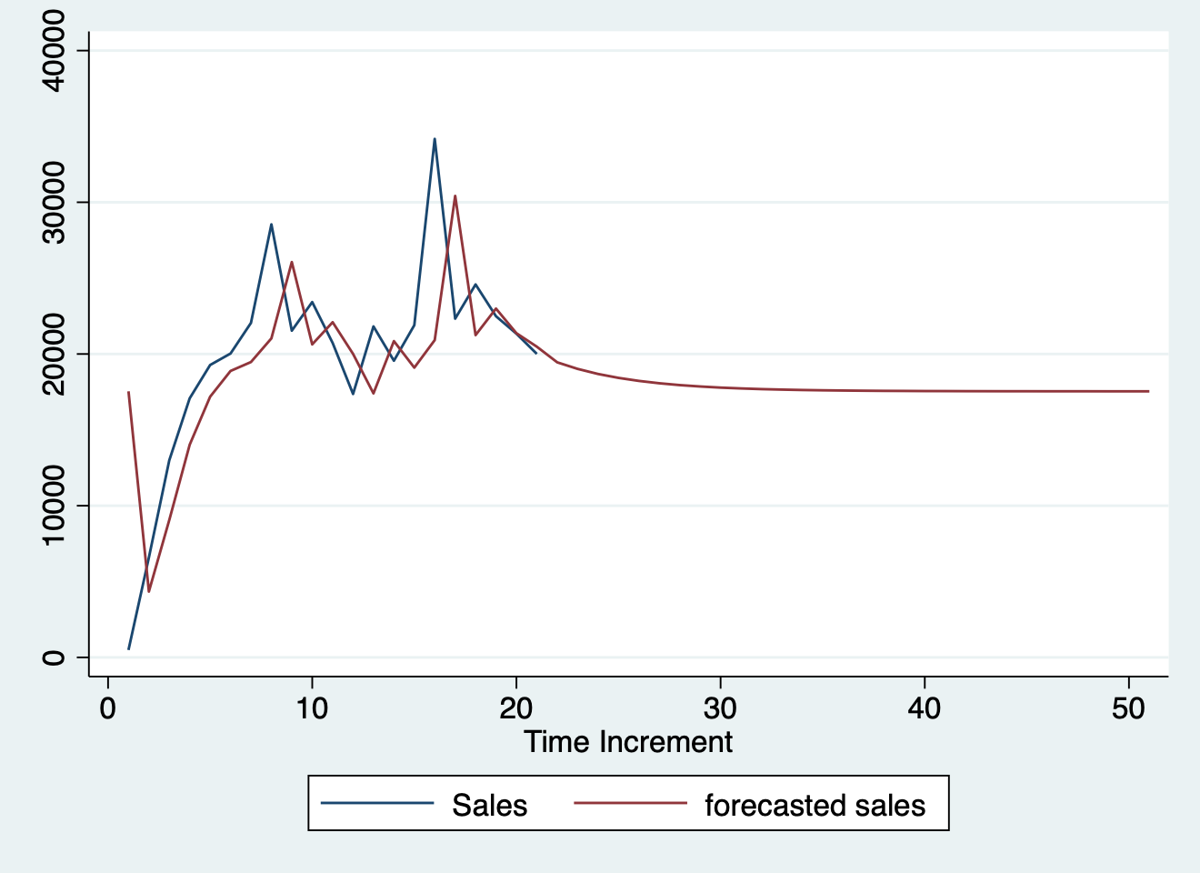
Python
from pandas import DataFrame
import statsmodels.api as sm
import matplotlib as plot

Stock_Market = {'Year': [2017,2017,2017,2017,2017,
                         2017,2017,2017,2017,2017,
                         2017,2017,2016,2016,2016,
                         2016,2016,2016,2016,2016,
                         2016,2016,2016,2016],
                'Month': [12, 11,10,9,8,7,6,5,4,
                          3,2,1,12,11,10,9,8,7,6,
                          5,4,3,2,1],
                'Interest_Rate':[2.75,2.5,2.5,2.5,2.5,2.5,
                                 2.5,2.25,2.25,2.25,2,2,2,1.75,1.75,
                                 1.75,1.75,1.75,1.75,1.75,1.75,1.75,1.75,1.75],
                'Unemployment_Rate':[5.3,5.3,5.3,5.3,5.4,5.6,
                                     5.5,5.5,5.5,5.6,5.7,5.9,6,5.9,5.8,6.1,
                                     6.2,6.1,6.1,6.1,5.9,6.2,6.2,6.1],
                'Stock_Index_Price': [1464,1394,1357,1293,1256,1254,1234,1195,1159,1167,1130,
                                      1075,1047,965,943,958,971,949,884,866,876,822,704,719]
                }

df = DataFrame(Stock_Market,columns=['Year','Month','Interest_Rate',
                                     'Unemployment_Rate','Stock_Index_Price'])

X = df[['Interest_Rate','Unemployment_Rate']]

# here we have 2 variables for the multiple linear regression. If you just want to use one variable for simple linear regression, then use X = df['Interest_Rate'] for example

Y = df['Stock_Index_Price']

X = sm.add_constant(X) # adding a constant

model = sm.OLS(Y, X).fit()
predictions = model.predict(X)

print_model = model.summary()
print(print_model)
#>                             OLS Regression Results
#> ==============================================================================
#> Dep. Variable:      Stock_Index_Price   R-squared:                       0.898
#> Model:                            OLS   Adj. R-squared:                  0.888
#> Method:                 Least Squares   F-statistic:                     92.07
#> Date:                Sat, 10 Oct 2026   Prob (F-statistic):           4.04e-11
#> Time:                        02:36:19   Log-Likelihood:                -134.61
#> No. Observations:                  24   AIC:                             275.2
#> Df Residuals:                      21   BIC:                             278.8
#> Df Model:                           2
#> Covariance Type:            nonrobust
#> =====================================================================================
#>                         coef    std err          t      P>|t|      [0.025      0.975]
#> -------------------------------------------------------------------------------------
#> const              1798.4040    899.248      2.000      0.059     -71.685    3668.493
#> Interest_Rate       345.5401    111.367      3.103      0.005     113.940     577.140
#> Unemployment_Rate  -250.1466    117.950     -2.121      0.046    -495.437      -4.856
#> ==============================================================================
#> Omnibus:                        2.691   Durbin-Watson:                   0.530
#> Prob(Omnibus):                  0.260   Jarque-Bera (JB):                1.551
#> Skew:                          -0.612   Prob(JB):                        0.461
#> Kurtosis:                       3.226   Cond. No.                         394.
#> ==============================================================================
#>
#> Notes:
#> [1] Standard Errors assume that the covariance matrix of the errors is correctly specified.
R
Stata
sysuse auto2, clear
* parallel processing removed (invalid Stata syntax)
mfp: glm price mpg
twoway (fpfitci price mpg, estcmd(glm) fcolor(dkorange%20) alcolor(%40))  || scatter price mpg, mcolor(dkorange) scale(0.75)
graph export "mfp.png", replace
#> . sysuse auto2, clear
#> (1978 automobile data)
#>
#> . * parallel processing removed (invalid Stata syntax)
#> . mfp: glm price mpg
#>
#> Deviance for model with all terms untransformed = 699.098, 74 observations
#>
#> Variable     Model (vs.)   Deviance  Dev diff.   P      Powers   (vs.)
#> ----------------------------------------------------------------------
#> mpg          Lin.   FP2     699.098     9.527  0.023+   1         -2 -2
#>              FP1            690.898     1.327  0.515    -2
#>              Final          690.898                     -2
#>
#>
#> Transformations of covariates:
#>
#> -> gen double Impg__1 = X^-2-.2204707671 if e(sample)
#>    (where: X = mpg/10)
#>
#> Final multivariable fractional polynomial model for price
#> --------------------------------------------------------------------
#>     Variable |    -----Initial-----          -----Final-----
#>              |   df     Select   Alpha    Status    df    Powers
#> -------------+------------------------------------------------------
#>          mpg |    4     1.0000   0.0500     in      2     -2
#> --------------------------------------------------------------------
#>
#> Generalized linear models                         Number of obs   =         74
#> Optimization     : ML                             Residual df     =         72
#>                                                   Scale parameter =   5.8e+164
#> Deviance         =  398426217.4                   (1/df) Deviance =    5533697
#> Pearson          =  398426217.4                   (1/df) Pearson  =    5533697
#>
#> Variance function: V(u) = 1                       [Gaussian]
#> Link function    : g(u) = u                       [Identity]
#>
#>                                                   AIC             =   9.390509
#> Log likelihood   = -345.4488489                   BIC             =   3.98e+08
#>
#> ------------------------------------------------------------------------------
#>              |                 OIM
#>        price | Coefficient  std. err.      z    P>|z|     [95% conf. interval]
#> -------------+----------------------------------------------------------------
#>      Impg__1 |   13163.85   2640.678     4.99   0.000     7988.216    18339.48
#>        _cons |   5538.395   468.7565    11.82   0.000     4619.649    6457.141
#> ------------------------------------------------------------------------------
#> Deviance = 690.898.
#>
#> . twoway (fpfitci price mpg, estcmd(glm) fcolor(dkorange%20) alcolor(%40))  || scatter price mpg, mcolor(dkorange) scale(0.75)
#>
#> . graph export "mfp.png", replace
#> file /Users/zad/LessLikely/my-quarto-site/statistics/mfp.png saved as PNG format
#>
#> .
#> OMP: Warning #96: Cannot form a team with 2 threads, using 1 instead.
#> OMP: Hint Consider unsetting KMP_DEVICE_THREAD_LIMIT (KMP_ALL_THREADS), KMP_TEAMS_THREAD_LIMIT, and OMP_THREAD_LIMIT (if any are set).
clear
set obs 100
/**
Generate variables from a normal distribution like before
*/
generate x = rnormal(0, 1)
generate y = rnormal(0, 1)
/**
We set up our model here

*/
* parallel processing removed (invalid Stata syntax)
bayesmh y x, likelihood(normal({var})) prior({var}, normal(0, 10)) ///
prior({y:}, normal(0, 10)) rseed(1031) saving(coutput_pred, replace) mcmcsize(1000)
/**
We use the bayespredict command to make predictions from the model
*/
bayespredict (mean:@mean({_resid})) (var:@variance({_resid})), ///
rseed(1031) saving(coutput_pred, replace)
/**
Then we calculate the posterior predictive P-values
*/
bayesstats ppvalues {mean} using coutput_pred
#> . clear
#>
#> . set obs 100
#> Number of observations (_N) was 0, now 100.
#>
#> . /**
#> > Generate variables from a normal distribution like before
#> > */
#> . generate x = rnormal(0, 1)
#>
#> . generate y = rnormal(0, 1)
#>
#> . /**
#> > We set up our model here
#> >
#> > */
#> . * parallel processing removed (invalid Stata syntax)
#> . bayesmh y x, likelihood(normal({var})) prior({var}, normal(0, 10)) ///
#> > prior({y:}, normal(0, 10)) rseed(1031) saving(coutput_pred, replace) mcmcsize(1000)
#>
#> Burn-in ...
#> Simulation ...
#>
#> Model summary
#> ------------------------------------------------------------------------------
#> Likelihood:
#>   y ~ normal(xb_y,{var})
#>
#> Priors:
#>   {y:x _cons} ~ normal(0,10)                                               (1)
#>         {var} ~ normal(0,10)
#> ------------------------------------------------------------------------------
#> (1) Parameters are elements of the linear form xb_y.
#>
#> Bayesian normal regression                       MCMC iterations  =      3,500
#> Random-walk Metropolis–Hastings sampling         Burn-in          =      2,500
#>                                                  MCMC sample size =      1,000
#>                                                  Number of obs    =        100
#>                                                  Acceptance rate  =      .2108
#>                                                  Efficiency:  min =   .0003942
#>                                                               avg =     .03501
#> Log marginal-likelihood = -148.08937                          max =     .06667
#>
#> ------------------------------------------------------------------------------
#>              |                                                Equal-tailed
#>              |      Mean   Std. dev.     MCSE     Median  [95% cred. interval]
#> -------------+----------------------------------------------------------------
#> y            |
#>            x | -.0048402   .1478623   .018108   .0259349  -.2962946   .2314111
#>        _cons |  .0108184    .140924   .022873   .0353712  -.2307058   .3144511
#> -------------+----------------------------------------------------------------
#>          var |  .9598697   .1379683   .219753   .9544686   .7353375   1.304321
#> ------------------------------------------------------------------------------
#>
#> file coutput_pred.dta saved.
#>
#> . /**
#> > We use the bayespredict command to make predictions from the model
#> > */
#> . bayespredict (mean:@mean({_resid})) (var:@variance({_resid})), ///
#> > rseed(1031) saving(coutput_pred, replace)
#>
#> Computing predictions ...
#>
#> file coutput_pred.dta saved.
#> file coutput_pred.ster saved.
#>
#> . /**
#> > Then we calculate the posterior predictive P-values
#> > */
#> . bayesstats ppvalues {mean} using coutput_pred
#>
#> Posterior predictive summary   MCMC sample size =     1,000
#>
#> -----------------------------------------------------------
#>            T |      Mean   Std. dev.  E(T_obs)  P(T>=T_obs)
#> -------------+---------------------------------------------
#>         mean |  .0037801   .0936636   .0625852           .3
#> -----------------------------------------------------------
#> Note: P(T>=T_obs) close to 0 or 1 indicates lack of fit.
#>
#> .
#> OMP: Warning #96: Cannot form a team with 2 threads, using 1 instead.
#> OMP: Hint Consider unsetting KMP_DEVICE_THREAD_LIMIT (KMP_ALL_THREADS), KMP_TEAMS_THREAD_LIMIT, and OMP_THREAD_LIMIT (if any are set).library(lme4)
library(simr)
# Toy model
fm = lmer(y ~ x + (x | g), data = simdata)
# Extend sample size of `g`
fm_extended_g = extend(fm, along = 'g', n = 4)
# 4 levels of g
pwcurve_4g = powerCurve(fm_extended_g, fixed('x'), along = 'g', breaks = 4,
nsim = 50, seed = 123,
# No progress bar
progress = FALSE)
# 6 levels of g
# Create a destination object using any of the power curves above.
all_pwcurve = pwcurve_4g
# Combine results
all_pwcurve$ps = c(pwcurve_4g$ps[1])
# Combine the different numbers of levels.
all_pwcurve$xval = c(pwcurve_4g$nlevels)
print(all_pwcurve)
#> Power for predictor 'x', (95% confidence interval),
#> by number of levels in g:
#> 4: 44.00% (29.99, 58.75) - 40 rows
#>
#> (0 errors, 1 warning, 40 messages)
#>
#> Time elapsed: 0 h 0 m 6 s
plot(all_pwcurve, xlab = 'Levels of g')
DataCamp notebooks:
- https://www.datacamp.com/datalab/w/2c40d510-1d81-4078-8ae3-9dcdd8f2a21b/print-notebook/notebook.ipynb
- https://www.datacamp.com/datalab/w/2c40d510-1d81-4078-8ae3-9dcdd8f2a21b/edit#welcome-environment
- https://www.datacamp.com/datalab/w/bf3f12b6-9b15-400f-8f0e-674b33b29cbe/print-report/notebook.ipynb#1-load-your-data
- https://www.datacamp.com/datalab/w/2c40d510-1d81-4078-8ae3-9dcdd8f2a21b/edit#considered-exemption


Webmentions
Replies, likes, and mentions from around the web, tracked via Webmention.io. What’s a webmention?
Comments