install.packages("concurve")
library("concurve")Tables, Graphs, and Computations from Rafi & Greenland (2020)
This post goes through the R code and logic that was used to construct the figures and concepts in Rafi & Greenland (2020) BMC MRM.
Keywords
p-value, p-value function, confidence curve, confidence distribution
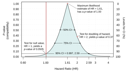
The following post provides some of the code that was used to construct the figures and tables from Rafi & Greenland, 20201. An enhanced PDF version of the paper can be found here. For further discussion of the computations, see the appendix of the main paper, along with our technical supplement.2
Disclaimer: I am responsible for all the code and mistakes below, and none of them can be attributed to my coauthors or my fellow package developers.
In order to recreate the functions, I would recommend installing the latest version of concurve from CRAN, as it has patched some issues with graphing when the outcome is binary. Use the script below to get the latest version and load the R package. A number of other R packages are also used in this post, which are listed below.
Valid -values Are Uniform Under the Null Model
Here we show that valid -values have specific properties, when the null model is true. We first generate two variables (, ) that come from the same normal distribution with a of 0 and of 1, each with a total of 1000 observations. We assume that there is no relationship between these two variables. We run a simple t-test between and and iterate this 100000 times and compute 100000 -values to see the overall distribution of the -values, which we then plot using a histogram./
RNGkind(kind = "L'Ecuyer-CMRG")
set.seed <- 1031
n.sim <- 100
t.sim <- numeric(n.sim)
n.samp <- 1000

for (i in 1:n.sim) {
    X <- rnorm(n.samp, mean = 0, sd = 1)
    Y <- rnorm(n.samp, mean = 0, sd = 1)
    df <- data.frame(X, Y)
    t <- t.test(X, Y, data = df)
    t.sim[i] <- t[[3]]
}

ggplot(NULL, aes(x = t.sim)) + geom_histogram(bins = 30, col = "black",
    fill = "#99c7c7", alpha = 0.25) + labs(title = "Distribution of P-values Under the Null",
    x = "P-value") + scale_x_continuous(breaks = seq(0, 1, 0.1)) +
    theme_bw()
This can also be shown using the TeachingDemos R package, which has a function dedicated to showing this phenomenon.
library("TeachingDemos")
RNGkind(kind = "L'Ecuyer-CMRG")
set.seed <- 1031
obs_p <- Pvalue.norm.sim(n = 1000, mu = 0, mu0 = 0, sigma = 1,
    sigma0 = 1, test = "t", alternative = "two.sided", alpha = 0.05,
    B = 1e+05)
ggplot(NULL, aes(x = obs_p)) + geom_histogram(bins = 30, col = "black",
    fill = "#99c7c7", alpha = 0.25) + labs(title = "Distribution of P-values Under the Null",
    x = "P-value") + scale_x_continuous(breaks = seq(0, 1, 0.1)) +
    theme_bw()
As you can see, when the null model is true, the distribution of -values is uniform. Valid -values are uniform under the null hypothesis and their corresponding -values are exponentially distributed. We run the same simulation as before, but then convert the obtained -values into -values, to see how they are distributed.
RNGkind(kind = "L'Ecuyer-CMRG")
set.seed <- 1031
n.sim <- 100
t.sim <- numeric(n.sim)
n.samp <- 1000

for (i in 1:n.sim) {
    X <- rnorm(n.samp, mean = 0, sd = 1)
    Y <- rnorm(n.samp, mean = 0, sd = 1)
    df <- data.frame(X, Y)
    t <- t.test(X, Y, data = df)
    t.sim[i] <- t[[3]]
}

ggplot(NULL, aes(x = -log2(t.sim))) + geom_histogram(bins = 30,
    col = "black", fill = "#d46c5b", alpha = 0.5) + labs(title = "Distribution of S-values Under the Null",
    x = "S-value (Bits of Information)") + theme_bw()
Posterior Predictive -values
Despite the name, posterior predictive -values are not considered valid frequentist -values because they do not meet the uniformity criterion, instead they are pulled towards the parameter value 0.5. For further discussion, see our technical supplement along with Greenland (2019) for comprehensive theoretical discussions.2, 3
A quick excerpt from our main paper and the technical supplement explains why this is not the case,
As discussed in the Supplement, in Bayesian settings one may see certain -values that are not valid frequentist -values, the primary example being the posterior predictive -value4;5; unfortunately, the negative logs of such invalid -values do not measure surprisal at the statistic given the model, and so are not valid -values.
The decision rule “reject H if ” will reject H 100% of the time under sampling from a model M obeying H (i.e., the Type-1 error rate of the test will be ) provided the random variable corresponding to is valid (uniform under the model M used to compute it), but not necessarily otherwise6. This is one reason why frequentist writers reject invalid -values (such as posterior predictive -values, which highly concentrate around 0.50) and devote considerable technical coverage to uniform -values6;5;4. A valid -value (“U-value”) translates into an exponentially distributed -value with a mean of 1 nat or bits where is the base of the natural logs.
Uniformity is also central to the “refutational information” interpretation of the -value used here, for it is necessary to ensure that the -value from which is derived is in fact the percentile of the observed value of the test statistic in the distribution of the statistic under M, thus making small surprising under M and making the corresponding degree of surprise. Because posterior predictive -values do not translate into sampling percentiles of the statistic under the hypothesis (in fact, they are pulled toward 0.5 from the correct percentiles)5;4, the resulting negative log does not measure surprisal at the statistic given M, and so is not a valid -value in our terms.
And indeed, we can show this phenomenon below with simulations. Here we fit a simple Bayesian regression model with a weakly informative prior normal(0, 10) using rstanarm, where both the predictor and response variable come from the same distribution and have the same location and scale parameters (, . We then calculate the observed test statistics, along with their distributions, and convert them into posterior predictive -values and plot them using Bayesplot functions. Then, we iterate this 1000 times to examine the distribution of posterior predictive -values and compare them to standard -values that are known to be uniform.
But first, we’ll generate the distribution of the test statistic from one model.
library("bayesplot")
library("rstan")
library("rstanarm")
rstan_options(auto_write = TRUE)
options(mc.cores = 4)
teal <- c("#99c7c7")
color_scheme_set("teal")
RNGkind(kind = "L'Ecuyer-CMRG")
n.samp <- 100
X <- rnorm(n.samp, mean = 0, sd = 1)
Y <- rnorm(n.samp, mean = 0, sd = 1)
df <- data.frame(X, Y)
mod1 <- stan_glm(Y ~ X, data = df, chains = 1, cores = 4, refresh = 0,
    prior = normal(0, 10))
#> Error in `if (!prior_dist_name %in% unlist(ok_dists)) ...`:
#> ! argument is of length zero
yrep <- posterior_predict(mod1)
#> Error:
#> ! object 'mod1' not found

h <- ppc_stat(Y, yrep, stat = "median", freq = TRUE, binwidth = 0.01) +
    labs(title = "Distribution of Posterior Test Statistic") +
    theme_bw() + yaxis_text(on = TRUE)
#> Error:
#> ! object 'yrep' not found

values_all <- h[["plot_env"]][["T_yrep"]]
#> Error:
#> ! object 'h' not found
prob_to_find <- h[["plot_env"]][["T_y"]]
#> Error:
#> ! object 'h' not found
quantInv <- function(distr, value) ecdf(distr)(value)
posterior_p_value <- quantInv(values_all, prob_to_find)
#> Error:
#> ! object 'values_all' not found

l <- ppc_stat_2d(Y, yrep) + theme_bw() + labs(title = "Distribution of Posterior Test Statistic")
#> Error:
#> ! object 'yrep' not found

plot(h)
#> Error in `h()`:
#> ! error in evaluating the argument 'x' in selecting a method for function 'plot': object 'h' not found
plot(l)
#> Error in `h()`:
#> ! error in evaluating the argument 'x' in selecting a method for function 'plot': object 'l' not foundprint(prob_to_find)
#> Error in `h()`:
#> ! error in evaluating the argument 'x' in selecting a method for function 'print': object 'prob_to_find' not foundThe above is the posterior predictive test statistic for one model, along with it’s distribution. Now let’s iterate this process, convert them into posterior predictive -values, and generate their distribution.
rstan_options(auto_write = TRUE)
options(mc.cores = 4)
RNGkind(kind = "L'Ecuyer-CMRG")
set.seed <- 1031
n.sim <- 100
ppp <- numeric(n.sim)
n.samp <- 1000

quantInv <- function(distr, value) ecdf(distr)(value)

for (i in 1:length(ppp)) {
    X <- rnorm(n.samp, mean = 0, sd = 1)
    Y <- rnorm(n.samp, mean = 0, sd = 1)
    df <- data.frame(X, Y)
    mod1 <- stan_glm(Y ~ X, data = df, chains = 1, cores = 4,
        iter = 1000, refresh = 0, prior = normal(0, 10))
    yrep <- posterior_predict(mod1)
    h <- ppc_stat(Y, yrep, stat = "median")
    values_all <- h[["plot_env"]][["T_yrep"]]
    prob_to_find <- h[["plot_env"]][["T_y"]]
    posterior_p_value <- quantInv(values_all, prob_to_find)
    ppp[i] <- posterior_p_value
}
#> Error in `if (!prior_dist_name %in% unlist(ok_dists)) ...`:
#> ! argument is of length zero

ggplot(NULL, aes(x = ppp)) + geom_histogram(bins = 30, col = "black",
    fill = "#99c7c7", alpha = 0.25) + labs(title = "Distribution of Posterior Predictive P-values",
    subtitle = "From Simulation of 1000 Simple Linear Regressions",
    x = "Posterior Predictive P-value") + scale_x_continuous(breaks = seq(0,
    1, 0.1)) + theme_bw()
We can also show this in Stata 16.1, using their new bayesstats ppvalues command which generates posterior predictive -values.
clear
set seed 1031
set obs 100

generate x = rnormal(0, 1)
generate y = rnormal(0, 1)

* Bayesian linear regression of y on x, mirroring the rstanarm model.
* Stata parameterizes the normal() prior by VARIANCE, so rstanarm's
* normal(0, sd = 10) is normal(0, 100) here. {y:} puts the prior on all
* regression coefficients including the intercept -- bayesmh requires a
* prior for every parameter. The variance gets a proper inverse-gamma
* prior; a normal prior is invalid for {var} (its support includes
* negative values).
bayesmh y x, likelihood(normal({var}))  ///
    prior({y:}, normal(0, 100))         ///
    prior({var}, igamma(0.01, 0.01))    ///
    rseed(1031) mcmcsize(1000)          ///
    saving(bmh_sim, replace)

* Simulate replicated outcomes from the posterior predictive
* distribution. This must be saved to a DIFFERENT file than the
* bayesmh simulation dataset above.
bayespredict {_ysim}, rseed(1031) saving(bmh_pred, replace)

* Posterior predictive p-values for test statistics of the replicated
* outcome. (The R analog uses the median; @median is not a built-in
* bayespredict/bayesstats function, so we use the mean and variance,
* matching the worked example in [BAYES] bayesstats ppvalues.)
bayesstats ppvalues (tmean:@mean({_ysim})) (tvar:@variance({_ysim})) ///
    using bmh_pred
#> Number of observations (_N) was 0, now 100.
#>
#>
#>
#>
#> Burn-in ...
#> Simulation ...
#>
#> Model summary
#> ------------------------------------------------------------------------------
#> Likelihood:
#>   y ~ normal(xb_y,{var})
#>
#> Priors:
#>   {y:x _cons} ~ normal(0,100)                                              (1)
#>         {var} ~ igamma(0.01,0.01)
#> ------------------------------------------------------------------------------
#> (1) Parameters are elements of the linear form xb_y.
#>
#> Bayesian normal regression                       MCMC iterations  =      3,500
#> Random-walk Metropolis–Hastings sampling         Burn-in          =      2,500
#>                                                  MCMC sample size =      1,000
#>                                                  Number of obs    =        100
#>                                                  Acceptance rate  =      .2428
#>                                                  Efficiency:  min =    .001044
#>                                                               avg =     .04252
#> Log marginal-likelihood = -153.90987                          max =     .08305
#>
#> ------------------------------------------------------------------------------
#>              |                                                Equal-tailed
#>              |      Mean   Std. dev.     MCSE     Median  [95% cred. interval]
#> -------------+----------------------------------------------------------------
#> y            |
#>            x |  .0115139   .1551555   .017026   .0145751  -.2995666   .3470796
#>        _cons |  .1022613    .137549   .020865   .1348998  -.2513679   .3455865
#> -------------+----------------------------------------------------------------
#>          var |  .9643251   .1503727    .14715   .9896135   .7582507   1.360154
#> ------------------------------------------------------------------------------
#>
#> file bmh_sim.dta saved.
#>
#>
#> Computing predictions ...
#>
#> file bmh_pred.dta saved.
#> file bmh_pred.ster saved.
#>
#>
#> Posterior predictive summary   MCMC sample size =     1,000
#>
#> -----------------------------------------------------------
#>            T |      Mean   Std. dev.  E(T_obs)  P(T>=T_obs)
#> -------------+---------------------------------------------
#>        tmean |  .0550687   .1146021   .0206952         .632
#>         tvar |  .9896307   .2164376   .9710317         .484
#> -----------------------------------------------------------
#> Note: P(T>=T_obs) close to 0 or 1 indicates lack of fit.
#>
#> OMP: Warning #96: Cannot form a team with 2 threads, using 1 instead.
#> OMP: Hint Consider unsetting KMP_DEVICE_THREAD_LIMIT (KMP_ALL_THREADS), KMP_TEAMS_THREAD_LIMIT, and OMP_THREAD_LIMIT (if any are set).
As we can see from the R plot above, the test statistics are are generally concentrated around 0.5 and the distribution (as shown above via the R code) hardly resembles the uniform distribution of -value under the null model. Further, the base-2 log transformation of posterior predictive -values is not exponentially distributed, making them invalid -values in our terms.
ggplot(NULL, aes(x = (-log2(ppp)))) + geom_histogram(bins = 30,
    col = "black", fill = "#d46c5b", alpha = 0.25) + labs(title = "Distribution of -log2(Posterior Predictive P-values)",
    subtitle = "S-values Produced From Posterior Predictive P-values",
    x = "-log2(Posterior Predictive P-value)") + theme_bw()
#> Error in `geom_histogram()`:
#> ! Problem while computing stat.
#> ℹ Error occurred in the 1st layer.
#> Caused by error in `seq_len()`:
#> ! argument must be coercible to non-negative integer
Table 1: Some -values, -values, Maximum Likelihood Ratios, and Likelihood Ratio Statistics
Here, we look at some common -values, and how they correspond to other information statistics and likelihood measures.
pvalue <- c(0.99, 0.9, 0.5, 0.25, 0.1, 0.05, 0.025, 0.01, 0.005,
    1e-04, paste("5 sigma (~ 2.9 in 10 million)"), paste("1 in 100 million (GWAS)"),
    paste("6 sigma (~ 1 in a billion)"))

svalue <- round(c(-log2(c(0.99, 0.9, 0.5, 0.25, 0.1, 0.05, 0.025,
    0.01, 0.005, 1e-04)), 21.7, 26.6, 29.9), 2)

pvalue[1:10] <- formatC(pvalue[1:10], format = "e", digits = 2)

mlr <- round(c(1, 1.01, 1.26, 1.94, 3.87, 6.83, 12.3, 27.6, 51.4,
    1935, (5.2 * (10^5)), (1.4 * (10^7)), (1.3 * (10^8))), 2)

# likelihood ratio statistic

lr <- round(c(0.00016, 0.016, 0.45, 1.32, 2.71, 3.84, 5.02, 6.63,
    7.88, 15.1, 26.3, 32.8, 37.4), 2)

table1 <- data.frame(pvalue, svalue, mlr, lr)

colnames(table1) <- c("P-value (compatibility)", "S-value (bits)",
    "Maximum Likelihood Ratio", "Deviance Statistic 2ln(MLR)")

kbl(table1, format = "html", padding = 45, longtable = TRUE,
    color = "#777") %>%
    row_spec(row = 0, color = "#777", bold = T) %>%
    column_spec(column = 1:4, color = "#777", bold = F) %>%
    kable_classic(full_width = TRUE, html_font = "Cambria", lightable_options = "basic",
        font_size = 17, fixed_thead = list(enabled = F)) %>%
    footnote(general_title = "Abbreviations: ", title_format = "underline",
general = c("Table 1 $P$-values and binary $S$-values, with corresponding maximum-likelihood ratios (MLR) and deviance (likelihood-ratio) statistics for a simple test hypothesis H under background assumptions A"))| P-value (compatibility) | S-value (bits) | Maximum Likelihood Ratio | Deviance Statistic 2ln(MLR) |
|---|---|---|---|
| 0.99 | 0.01 | 1.00e+00 | 0.00 |
| 0.9 | 0.15 | 1.01e+00 | 0.02 |
| 0.5 | 1.00 | 1.26e+00 | 0.45 |
| 0.25 | 2.00 | 1.94e+00 | 1.32 |
| 0.1 | 3.32 | 3.87e+00 | 2.71 |
| 0.05 | 4.32 | 6.83e+00 | 3.84 |
| 0.025 | 5.32 | 1.23e+01 | 5.02 |
| 0.01 | 6.64 | 2.76e+01 | 6.63 |
| 0.005 | 7.64 | 5.14e+01 | 7.88 |
| 1e-04 | 13.29 | 1.94e+03 | 15.10 |
| 5 sigma (~ 2.9 in 10 million) | 21.70 | 5.20e+05 | 26.30 |
| 1 in 100 million (GWAS) | 26.60 | 1.40e+07 | 32.80 |
| 6 sigma (~ 1 in a billion) | 29.90 | 1.30e+08 | 37.40 |
| Abbreviations: | |||
| Table 1 $P$-values and binary $S$-values, with corresponding maximum-likelihood ratios (MLR) and deviance (likelihood-ratio) statistics for a simple test hypothesis H under background assumptions A |
For further discussion of 5 and 6 sigma cutoffs, see7.
Frequentist Interval Estimate Percentiles
Refer to Long-Run Coverage
Here we simulate a study where one group with 100 participants has an of 100 with a of 20 and the second group has the same number of participants but an average of 80 and a standard deviation of 20. We compare them using a Welch’s -test and generate 95% compatibility intervals several times, specifically 100 times, and then plot them. Since we know the mean difference is 20, we wish to see how often the interval estimates cover this true parameter value.
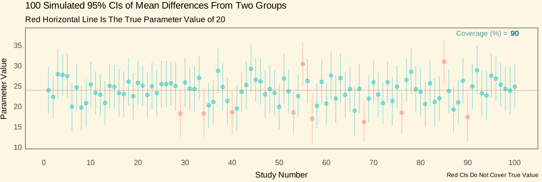
This shows that the intervals tend to vary simply as a result of randomness, and that the proper interpretation of the attached percentile is about long run coverage of the true parameter. However, this does not preclude interpretation of a single interval estimate from a study.8 As we write in the Replace unrealistic “confidence” claims with compatibility measures section of our paper.1
The fact that “confidence” refers to the procedure behavior, not the reported interval, seems to be lost on most researchers. Remarking on this subtlety, when Jerzy Neyman discussed his confidence concept in 1934 at a meeting of the Royal Statistical Society, Arthur Bowley replied, “I am not at all sure that the ‘confidence’ is not a confidence trick.”9. And indeed, 40 years later, Cox and Hinkley warned, “interval estimates cannot be taken as probability statements about parameters, and foremost is the interpretation ‘such and such parameter values are consistent with the data.’”8. Unfortunately, the word “consistency” is used for several other concepts in statistics, while in logic it refers to an absolute condition (of noncontradiction); thus, its use in place of “confidence” would risk further confusion.
To address the problems above, we exploit the fact that a 95% CI summarizes the results of varying the test hypothesis H over a range of parameter values, displaying all values for which > 0.0510 and hence < 4.32 bits3;11. Thus the CI contains a range of parameter values that are more compatible with the data than are values outside the interval, under the background assumptions3;12. Unconditionally (and thus even if the background assumptions are uncertain), the interval shows the values of the parameter which, when combined with the background assumptions, produce a test model that is “highly compatible” with the data in the sense of having less than 4.32 bits of information against it. We thus refer to CI as compatibility intervals rather than confidence intervals13;3;11; their abbreviation remains “CI.” We reject calling these intervals “uncertainty intervals,” because they do not capture uncertainty about background assumptions13.
Indeed, this also has to do with our paper on deemphasizing the model assumptions that are often behind common statistical outputs, and why it is necessary to treat them as uncertain, rather than given.14 For example, a 95% interval estimate is assumed to be free of bias in its construction, however, it’s coverage claims are no longer so, once there are systematic errors in play. Many of these common, classical statistical procedures are designed to deal with random variation, and less so with bias (a relatively new field, with shiny new methods).
Brown et al. (2017) Reanalysis
Taken from the Brown et al. data.15, 16
Here we take the reported statistics from the Brown et al. studies in order to run statistical tests of different alternative test hypotheses and use those results to construct various functions.
We calculate the standard errors from the point estimate and the confidence (compatibility) limits.
Table 2: -values, -values, and Likelihoods for Targeted Hypotheses About Hazard Ratios for Brown et al.
testhypothesis <- c("Halving of hazard", "No effect (null)",
    "Point estimate", "Doubling of hazard", "Tripling of hazard",
    "Quintupling of hazard")

hazardratios <- c(0.5, 1, 1.61, 2, 3, 5)
pvals <- c(1.6e-06, 0.05, 1, 0.37, 0.01, 3.2e-06)
svals <- round(-log2(pvals), 2)
mlr2 <- c((1 * 10^5), 6.77, 1, 1.49, 26.2, (5 * 10^4))
lr <- round(c(exp((((log(0.5/1.61))/se)^2)/(2)), exp((((log(1/1.61))/se)^2)/(2)),
    exp((((log(1.61/1.61))/se)^2)/(2)), exp((((log(2/1.61))/se)^2)/(2)),
    exp((((log(3/1.61))/se)^2)/(2)), exp((((log(5/1.61))/se)^2)/(2))),
    3)

LR <- formatC(lr, format = "e", digits = 2)

table2 <- data.frame(testhypothesis, hazardratios, pvals, svals,
    mlr2, LR)

colnames(table2) <- c("Test Hypothesis", "HR", "P-values", "S-values",
    "MLR", "LR")

kbl(table2, format = "html", padding = 45, longtable = TRUE,
    color = "#777") %>%
    row_spec(row = 0, color = "#777", bold = T) %>%
    column_spec(column = 1:6, color = "#777", bold = F) %>%
    kable_classic(full_width = TRUE, html_font = "Cambria", lightable_options = "basic",
font_size = 15, fixed_thead = list(enabled = F))| Test Hypothesis | HR | P-values | S-values | MLR | LR |
|---|---|---|---|---|---|
| Halving of hazard | 0.50 | 0.00 | 19.25 | 1.00e+05 | 1.02e+05 |
| No effect (null) | 1.00 | 0.05 | 4.32 | 6.77e+00 | 6.77e+00 |
| Point estimate | 1.61 | 1.00 | 0.00 | 1.00e+00 | 1.00e+00 |
| Doubling of hazard | 2.00 | 0.37 | 1.43 | 1.49e+00 | 1.49e+00 |
| Tripling of hazard | 3.00 | 0.01 | 6.64 | 2.62e+01 | 2.62e+01 |
| Quintupling of hazard | 5.00 | 0.00 | 18.25 | 5.00e+04 | 5.03e+04 |
Plot the point estimate and 95% compatibility interval
label <- c("Brown et al. (2017)\n JAMA", "Brown et al. (2017)\n J Clin Psychiatry")

point <- c(1.61, 1.7)
lower <- c(0.997, 1.1)
upper <- c(2.59, 2.6)

df <- data.frame(label, point, lower, upper)
Here we plot the 95% compatibility interval estimate reported from the high-dimensional propensity score analysis.
ggplot(data = df, mapping = aes(x = label, y = point, ymin = lower,
    ymax = upper, group = label)) + geom_pointrange(color = "#007C7C",
    size = 1.5, alpha = 0.4) + geom_hline(yintercept = 1, lty = 3,
    color = "#d46c5b", alpha = 0.5) + coord_flip() + scale_y_log10(breaks = scales::pretty_breaks(n = 10),
    limits = c(0.8, 4)) + labs(title = "Association Between Serotonergic Antidepressant Exposure
               \nDuring Pregnancy and Child Autism Spectrum Disorder",
    subtitle = "Reported 95% Compatibility Intervals From Primary Results",
    x = "Study", y = "Hazard Ratio (JAMA) +
            Adjusted Pooled Odds Ratio (J Clin Psychiatry)") +
    annotate(geom = "text", x = 1.5, y = 1, size = 5, label = "Null parameter value of 1",
        color = "#d46c5b", alpha = 0.75) + annotate(geom = "text",
    x = 2.2, y = 1.8, size = 5, label = "Point Estimate = 1.61,
           Lower Limit = 0.997, Upper Limit = 2.59",
    color = "#000000", alpha = 0.75) + annotate(geom = "text",
    x = 1.2, y = 1.8, size = 5, label = "Point Estimate = 1.7,
           Lower Limit = 1.1, Upper Limit = 2.6",
    color = "#000000", alpha = 0.75) + theme_light() + theme(axis.text.y = element_text(angle = 90,
    hjust = 1, size = 13)) + theme(axis.text.x = element_text(size = 13)) +
    theme(title = element_text(size = 13))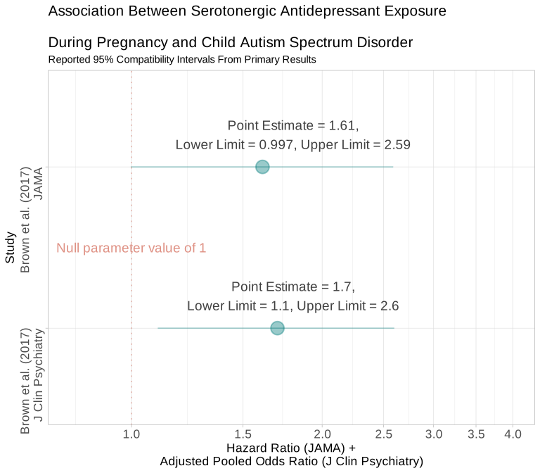
Once again, the authors reported that15
In the 2837 pregnancies (7.9%) exposed to antidepressants, 2.0% (95% CI, 1.6%-2.6%) of children were diagnosed with autism spectrum disorder. Risk of autism spectrum disorder was significantly higher with serotonergic antidepressant exposure (4.51 exposed vs 2.03 unexposed per 1000 person-years; between-group difference, 2.48 95% CI, 2.33-2.62 per 1000 person-years) in crude (HR, 2.16 95% CI, 1.64-2.86) and multivariable-adjusted analyses (HR, 1.59 95% CI, 1.17-2.17) (Table 2). After inverse probability of treatment weighting based on the HDPS, the association was not significant (HR, 1.61 95% CI, 0.997-2.59) (Table 2).
and concluded with
In children born to mothers receiving public drug coverage in Ontario, Canada, in utero serotonergic antidepressant exposure compared with no exposure was not associated with autism spectrum disorder in the child. Although a causal relationship cannot be ruled out, the previously observed association may be explained by other factors.
We will show using the graphical and tabular summaries below, why a more nuanced summary such as,
“After HDPS adjustment for confounding, a 61% hazard elevation remained; however, under the same model, every hypothesis from no elevation up to a 160% hazard increase had > 0.05; Thus, while quite imprecise, these results are consistent with previous observations of a positive association between serotonergic antidepressant prescriptions and subsequent ASD. Because the association may be partially or wholly due to uncontrolled biases, further evidence will be needed for evaluating what, if any, proportion of it can be attributed to causal effects of prenatal serotonergic antidepressant use on ASD incidence.”
would have been far more appropriate, as we discuss in our paper.1
-value and -value Functions
In order to use this information to construct a -value function, we can use the concurve functions.
library("concurve")We enter the reported point estimates and compatibility limits and produce all possible intervals + -values + -values. This is calculated assuming normal approximations with the curve_rev() function.
curve1 <- curve_rev(point = 1.61, LL = 0.997, UL = 2.59, measure = "ratio")It is stored in the object curve1.
We can generate a table of the relevant statistics from this reanalysis, similar to the table from above, but this time using the concurve function, curve_table(), but this time it will give us interval estimates of various percentiles (%, %, %, %, etc.). These are in turn used to construct the entire confidence (compatibility) distribution or -value function.
kbl(curve_table(curve1[[1]]), format = "html", padding = 45,
    longtable = TRUE, color = "#777", row.names = F, col.names = colnames(curve_table(curve1[[1]]))) %>%
    row_spec(row = 0, color = "#777", bold = T) %>%
    column_spec(column = 1:7, color = "#777", bold = F) %>%
    kable_classic(full_width = TRUE, html_font = "Cambria", lightable_options = "basic",
        font_size = 17, fixed_thead = list(enabled = F)) %>%
    footnote(general_title = c("Table of Statistics for Various Interval Estimate Percentiles"),
general = " ")| Lower Limit | Upper Limit | Interval Width | Interval Level (%) | CDF | P-value | S-value (bits) |
|---|---|---|---|---|---|---|
| 1.490 | 1.74 | 0.250 | 25.0 | 0.625 | 0.750 | 0.415 |
| 1.366 | 1.90 | 0.531 | 50.0 | 0.750 | 0.500 | 1.000 |
| 1.217 | 2.13 | 0.914 | 75.0 | 0.875 | 0.250 | 2.000 |
| 1.178 | 2.20 | 1.021 | 80.0 | 0.900 | 0.200 | 2.322 |
| 1.134 | 2.29 | 1.152 | 85.0 | 0.925 | 0.150 | 2.737 |
| 1.079 | 2.40 | 1.325 | 90.0 | 0.950 | 0.100 | 3.322 |
| 0.999 | 2.60 | 1.596 | 95.0 | 0.975 | 0.050 | 4.322 |
| 0.933 | 2.78 | 1.846 | 97.5 | 0.988 | 0.025 | 5.322 |
| 0.860 | 3.02 | 2.155 | 99.0 | 0.995 | 0.010 | 6.644 |
| Table of Statistics for Various Interval Estimate Percentiles | ||||||
Figure 3: -value (Compatibility) Function
Plot the -value (Compatibility) function of the Brown et al. data
Now we plot the -value function from the data stored in curve1 using the ggcurve() function from concurve.
ggcurve(curve1[[1]], type = "c", measure = "ratio", nullvalue = c(1),
    levels = c(0.5, 0.75, 0.95)) + labs(title = expression(paste(italic(P),
    "-value (Compatibility) Function")), subtitle = expression(paste(italic(P),
    "-values for a range of hazard ratios (HR)")), x = "Hazard Ratio (HR)",
    y = expression(paste(italic(P), "-value"))) + geom_vline(xintercept = 1.61,
    lty = 1, color = "gray", alpha = 0.2) + geom_vline(xintercept = 2.59,
    lty = 1, color = "gray", alpha = 0.2) + theme(plot.title = element_text(size = 12),
    plot.subtitle = element_text(size = 11), axis.title.x = element_text(size = 12),
    axis.title.y = element_text(size = 12), text = element_text(size = 11))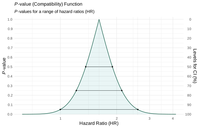
It is practically the same as the published version from Rafi & Greenland, 20201.
Cumulative Confidence (Compatibility Distribution)
Although we do not cover this figure in our paper, it is easy to construct using concurve's ggcurve() function by specifying type as “cdf” to see the median estimate within the confidence distribution. The horizontal line that meets at the curve, is approximately the same as the maximum at the -value function/confidence (compatibility) curve.
ggcurve(curve1[[2]], type = "cdf", measure = "ratio", nullvalue = c(1)) +
    labs(title = "P-values for a range of hazard ratios (HR)",
        subtitle = "Association Between Serotonergic Antidepressant Exposure
       \nDuring Pregnancy and Child Autism Spectrum Disorder",
        x = "Hazard Ratio (HR)", y = "Cumulative Compatibility") +
    theme(plot.title = element_text(size = 12), plot.subtitle = element_text(size = 11),
        axis.title.x = element_text(size = 12), axis.title.y = element_text(size = 12),
        text = element_text(size = 11))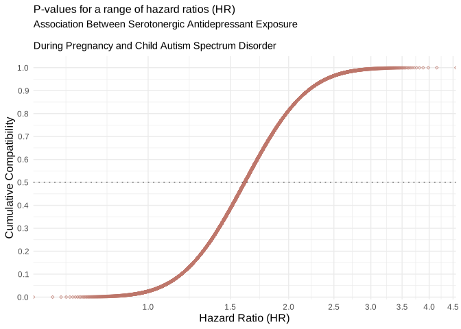
We will also calculate the likelihoods so that we can generate the corresponding likelihood functions.
We can also see how consistent these results are with previous studies conducted by the same research group, given the overlap of the functions, which can be compared using the plot_compare() function. Let’s compare the relative likelihood functions from both studies from this research group to see how consistent the results are.
plot_compare(data1 = lik1[[1]], data2 = lik2[[1]], type = "l1",
    measure = "ratio", nullvalue = TRUE, title = "Brown et al. 2017. J Clin Psychiatry. vs.
              \nBrown et al. 2017. JAMA.",
    subtitle = "J Clin Psychiatry: OR = 1.7, 1/6.83 LI: LL = 1.1, UL = 2.6
                         \nJAMA: HR = 1.61, 1/6.83 LI: LL = 0.997, UL = 2.59",
    xaxis = "Hazard Ratio / Odds Ratio") + theme(plot.title = element_text(size = 12),
    plot.subtitle = element_text(size = 11), axis.title.x = element_text(size = 12),
    axis.title.y = element_text(size = 12), text = element_text(size = 11))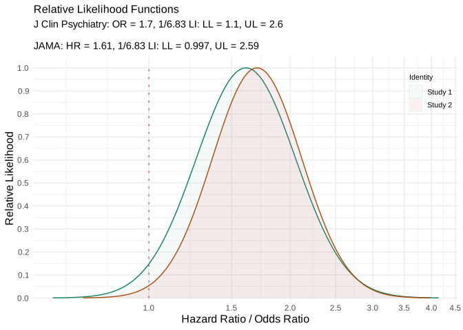
and the -value functions.
plot_compare(data1 = curve1[[1]], data2 = curve2[[1]], type = "c",
    measure = "ratio", nullvalue = TRUE, title = "Brown et al. 2017. J Clin Psychiatry. vs.
              \nBrown et al. 2017. JAMA.",
    subtitle = "J Clin Psychiatry: OR = 1.7, 1/6.83 LI: LL = 1.1, UL = 2.6
              \nJAMA: HR = 1.61, 1/6.83 LI: LL = 0.997, UL = 2.59",
    xaxis = "Hazard Ratio / Odds Ratio") + theme(plot.title = element_text(size = 12),
    plot.subtitle = element_text(size = 11), axis.title.x = element_text(size = 12),
    axis.title.y = element_text(size = 12), text = element_text(size = 11))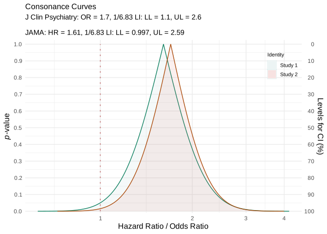
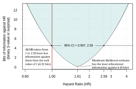
Figure 4: -value (Suprisal) Function
Plot the -value (Surprisal) function of the Brown et al. data with ggcurve()
ggcurve(data = curve1[[1]], type = "s", measure = "ratio", nullvalue = c(1),
    title = "S-value (Surprisal) Function", subtitle = "S-Values (surprisals) for a range of hazard ratios (HR)",
    xaxis = "Hazard Ratio", yaxis1 = "S-value (bits of information)") +
    theme(plot.title = element_text(size = 12), plot.subtitle = element_text(size = 11),
        axis.title.x = element_text(size = 12), axis.title.y = element_text(size = 12),
        text = element_text(size = 11))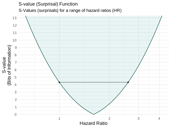
which is quite close to the figure from our paper.
Likelihood (Support) Functions
Here we provide the code to show how we constructed the likelihood functions from our paper, which are the supplementary figures found here (S1) and here (S2).
Calculate and Plot Likelihood (Support) Intervals.
Here we use the reported estimates to construct the -scores and standard errors, which are in turn used to compute the likelihoods.
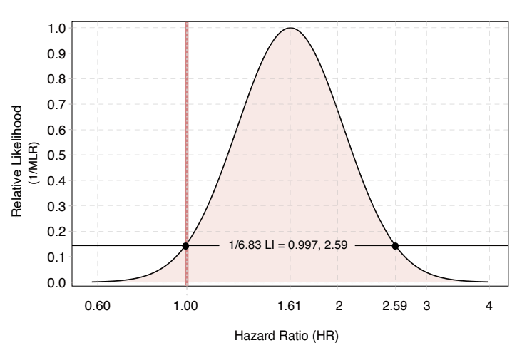
Figure S1: Relative Likelihood Function
We then standardize all the likelihoods by their maximum at the likelihood function,17 to produce relative likelihoods, likelihood intervals, and their corresponding relative likelihood function.18
support <- exp((-zscore^2)/2)

likfunction <- data.frame(hrvalues, zscore, support)

ggplot(data = likfunction, mapping = aes(x = hrvalues, y = support)) +
    geom_line() + geom_vline(xintercept = 1, lty = 3, color = "#d46c5b",
    alpha = 0.75) + geom_hline(yintercept = (1/6.83), lty = 1,
    color = "#333333", alpha = 0.05) + geom_ribbon(aes(x = hrvalues,
    ymin = min(support), ymax = support), fill = "#d46c5b", alpha = 0.1) +
    labs(title = "Relative Likelihood Function", subtitle = "Relative likelihoods for a range of hazard ratios",
        x = "Hazard Ratio (HR)", y = "Relative Likelihood \n1/MLR") +
    annotate(geom = "text", x = 1.65, y = 0.2, label = "1/6.83 LI = 0.997, 2.59",
        size = 4, color = "#000000") + theme_bw() + theme(plot.title = element_text(size = 12),
    plot.subtitle = element_text(size = 11), axis.title.x = element_text(size = 12),
    axis.title.y = element_text(size = 12), text = element_text(size = 11)) +
    scale_x_log10(breaks = scales::pretty_breaks(n = 10)) + scale_y_continuous(expand = expansion(mult = c(0.01,
    0.0125)), breaks = seq(0, 1, 0.1))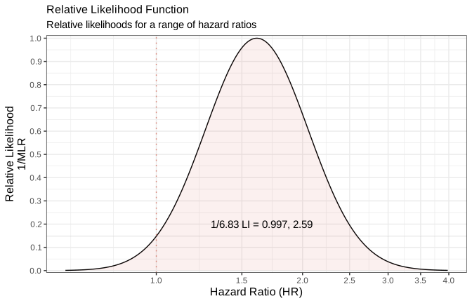
The likelihood interval corresponds to the 95% compatibility interval, as shown by the figure from our paper.
Below we use the calculated -scores to construct the log-likelihood function which is the upward-concave parabola =
support <- (zscore^2)/2

likfunction <- data.frame(hrvalues, zscore, support)

ggplot(data = likfunction, mapping = aes(x = hrvalues, y = support)) +
    geom_line() + geom_vline(xintercept = 1, lty = 3, color = "#d46c5b",
    alpha = 0.75) + geom_ribbon(aes(x = hrvalues, ymin = support,
    ymax = max(support)), fill = "#d46c5b", alpha = 0.1) + labs(title = "Log-Likelihood Function",
    subtitle = "Log-likelihoods for a range of hazard ratios",
    x = "Hazard Ratio (HR)", y = "ln(MLR)") + theme_bw() + theme(axis.title.x = element_text(size = 13),
    axis.title.y = element_text(size = 13)) + scale_x_log10(breaks = scales::pretty_breaks(n = 10)) +
    scale_y_continuous(expand = expansion(mult = c(0.01, 0.0125)),
        breaks = seq(0, 7, 1)) + theme(text = element_text(size = 15)) +
    theme(plot.title = element_text(size = 12), plot.subtitle = element_text(size = 12))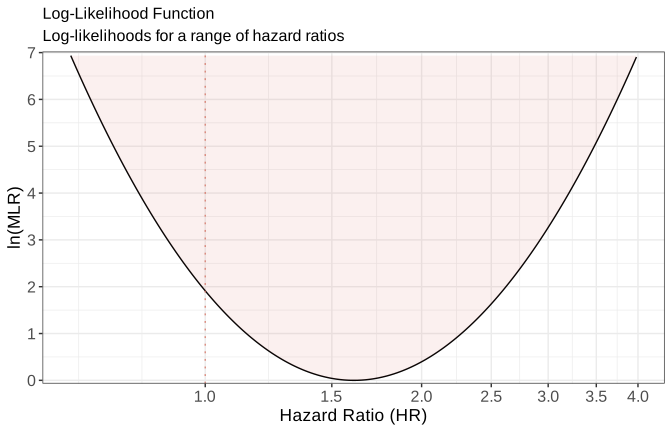
Figure S2: Deviance Function
Known as the deviance function, it is twice the log-likelihood, which maps to the -value function.
support <- (zscore^2)

likfunction <- data.frame(hrvalues, zscore, support)

ggplot(data = likfunction, mapping = aes(x = hrvalues, y = support)) +
    geom_line() + geom_vline(xintercept = 1, lty = 3, color = "#d46c5b",
    alpha = 0.75) + geom_hline(yintercept = 3.84, lty = 1, color = "#333333",
    alpha = 0.05) + geom_ribbon(aes(x = hrvalues, ymin = support,
    ymax = max(support)), fill = "#d46c5b", alpha = 0.1) + annotate(geom = "text",
    x = 1.65, y = 4.4, label = "1/6.83 LI = 0.997, 2.59", size = 4,
    color = "#000000") + theme_bw() + theme(plot.title = element_text(size = 12),
    plot.subtitle = element_text(size = 11), axis.title.x = element_text(size = 12),
    axis.title.y = element_text(size = 12), text = element_text(size = 11)) +
    scale_x_log10(breaks = scales::pretty_breaks(n = 10)) + scale_y_continuous(expand = expansion(mult = c(0.01,
    0.0125)), breaks = seq(0, 14, 2)) + labs(title = "Deviance Function",
    subtitle = "Deviance statistics for a range of hazard ratios",
    x = "Hazard Ratio (HR)", y = " Deviance Statistic \n2ln(MLR)")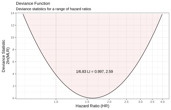
And the version from our paper can be found here.
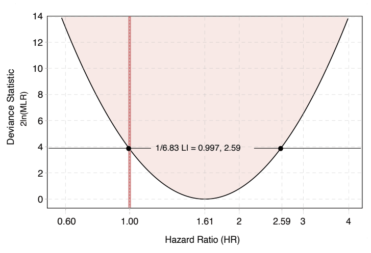
It is important to note that although we have calculated these likelihood functions manually here, they can also be generated easily using the curve_lik() function which takes inputs from the ProfileLikelihood R package. To see a further discussion, please see the following article, which gives several examples for a wide variety of models.
Further, we urge some caution. Although we endorse the construction and presentation of likelihood functions along with -value and -value functions, along with the tabulations, the use of pure likelihood methods has been highly controversial among some statisticians, with some going as far as to say that likelihood is blind although not all statisticians believe this, and have responded to such criticisms in kind, see discussants.19 Thus, we support providing both -value/-value and likelihood-based functions for a complete picture.
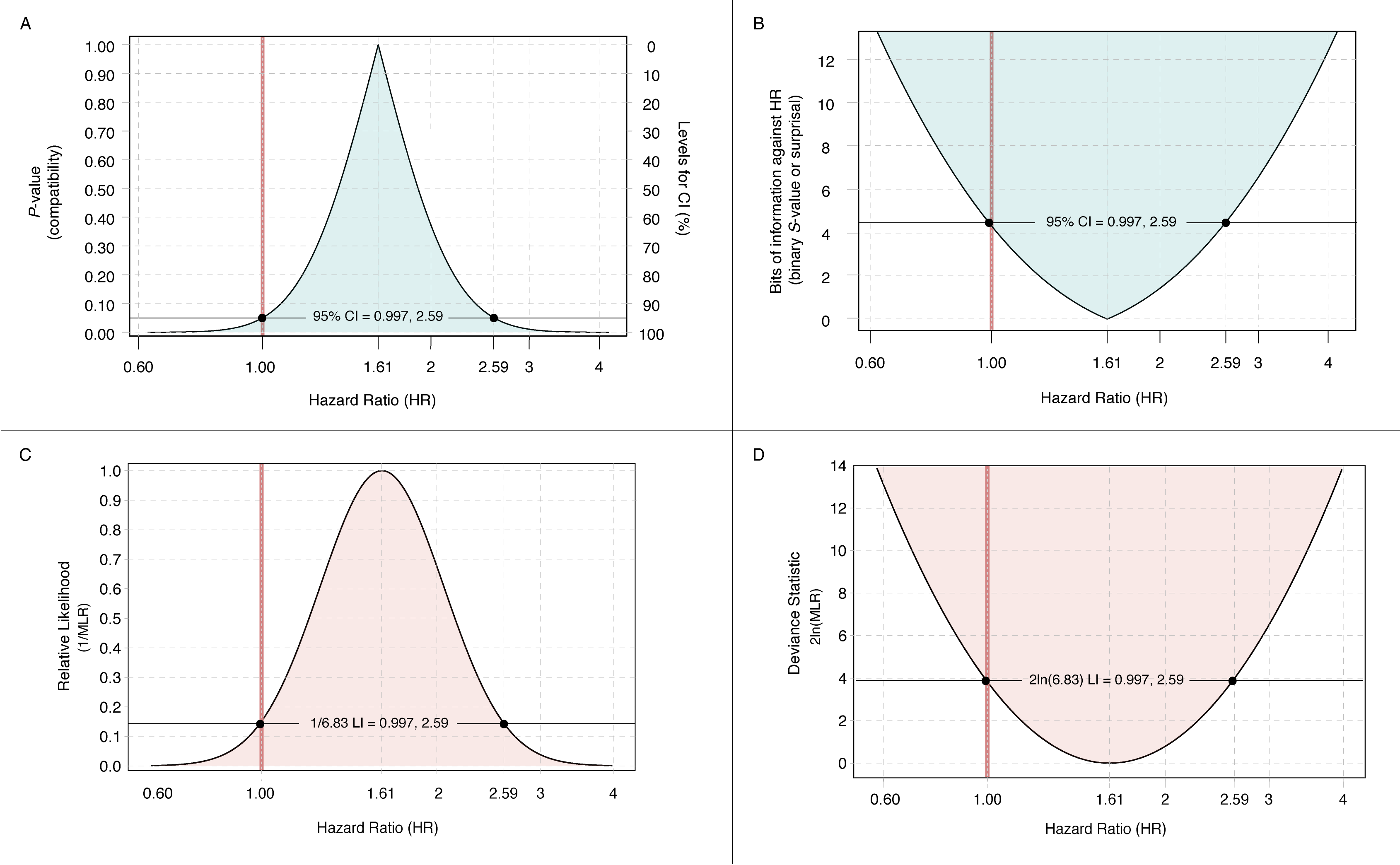
Indeed, we can see how they all easily map to one another when plotted side by side, with the following script.
A clearer plot comparing the four functions is seen below (click on the image to view in full).
Additional adjustments that were made to the figures from Rafi & Greenland, 20201 were done using Adobe Illustrator and Photoshop.
All errors are ours, and we welcome critical feedback and reporting of errors. To report possible errors in our analyses, please post it as a comment below or as a bug here. We will compile them onto a public errata, if any errors or flaws are reported to us.
Statistical Package Citations
Please remember to cite the R packages if you use any of the R scripts from above. The citation for our1 can be found below in the References section or it can be downloaded here for a reference manager.
Environment
The analyses were run on:
si <- sessionInfo()
print(si, RNG = TRUE, locale = TRUE)
#> R version 4.6.1 (2026-06-24)
#> Platform: aarch64-apple-darwin25.4.0
#> Running under: macOS Golden Gate 27.0.1
#>
#> Matrix products: default
#> BLAS:   /opt/homebrew/Cellar/openblas/0.3.34/lib/libopenblasp-r0.3.34.dylib
#> LAPACK: /opt/homebrew/Cellar/r/4.6.1/lib/R/lib/libRlapack.dylib;  LAPACK version 3.12.1
#>
#> Random number generation:
#>  RNG:     L'Ecuyer-CMRG
#>  Normal:  Inversion
#>  Sample:  Rejection
#>
#> locale:
#> [1] C.UTF-8/C.UTF-8/C.UTF-8/C/C.UTF-8/C.UTF-8
#>
#> time zone: America/New_York
#> tzcode source: internal
#>
#> attached base packages:
#>  [1] splines   grid      stats4    parallel  stats     graphics  grDevices
#>  [8] utils     datasets  methods   base
#>
#> other attached packages:
#>   [1] plotly_4.12.1         TSstudio_0.1.7        tfautograph_0.3.2
#>   [4] tfdatasets_2.18.0     keras_2.16.1          tensorflow_2.20.0
#>   [7] timetk_2.9.1          modeltime_1.3.5       workflowsets_1.1.1
#>  [10] workflows_1.3.0       tune_2.1.0            tailor_0.1.0
#>  [13] rsample_1.3.2         recipes_1.4.0         parsnip_1.6.1
#>  [16] modeldata_1.6.0       infer_1.1.0           dials_1.4.4
#>  [19] scales_1.4.0          tidymodels_1.5.0      xgboost_3.2.1.1
#>  [22] prophet_1.1.7         rlang_1.3.0           astsa_2.5
#>  [25] bayesforecast_1.0.5   smooth_4.5.2          greybox_2.0.9
#>  [28] glmnet_5.1            forecast_9.0.2        fable_0.5.0
#>  [31] fabletools_0.8.0      tsibbledata_0.4.1     tsibble_1.2.0
#>  [34] rstanarm_2.32.2       texPreview_2.1.0      tinytex_0.61
#>  [37] rmarkdown_2.32        brms_2.23.0           bootImpute_1.3.0
#>  [40] knitr_1.52            boot_1.3-32           JuliaCall_0.17.6
#>  [43] reshape2_1.4.5        ProfileLikelihood_1.3 ImputeRobust_1.3-1
#>  [46] gamlss_5.5-5          gamlss.dist_6.1-11    gamlss.data_6.0-7
#>  [49] mvtnorm_1.4-2         performance_0.18.2    summarytools_1.1.5
#>  [52] tidybayes_3.0.7       htmltools_0.5.9       Statamarkdown_1.1.0
#>  [55] car_3.1-5             carData_3.0-6         qqplotr_0.0.7
#>  [58] ggcorrplot_0.3.0      mitml_0.4-5           pbmcapply_1.5.1
#>  [61] Amelia_1.8.3          Rcpp_1.1.2            blogdown_1.24
#>  [64] doParallel_1.0.17     iterators_1.0.14      foreach_1.5.2
#>  [67] lattice_0.23-1        bayesplot_1.16.0      wesanderson_0.3.7
#>  [70] VIM_7.3.1             colorspace_2.1-4      here_1.0.2
#>  [73] progress_1.2.3        loo_2.10.1            mi_1.3.1
#>  [76] Matrix_1.7-6          broom_1.0.13          yardstick_1.4.0
#>  [79] svglite_2.2.2         Cairo_1.7-0           cowplot_1.2.0
#>  [82] mgcv_1.9-4            nlme_3.1-171          xfun_0.61
#>  [85] broom.mixed_0.2.9.7   reticulate_1.47.0     kableExtra_1.4.1
#>  [88] posterior_1.7.0       checkmate_2.3.4       parallelly_1.48.0
#>  [91] miceFast_0.9.1        randomForest_4.7-1.2  missForest_1.6.1
#>  [94] miceadds_3.20-10      quantreg_6.1          SparseM_1.84-2
#>  [97] MCMCpack_1.7-1        MASS_7.3-66           coda_0.19-4.1
#> [100] latex2exp_0.9.8       rstan_2.32.7          StanHeaders_2.39.1
#> [103] lubridate_1.9.5       forcats_1.0.1         stringr_1.6.0
#> [106] dplyr_1.2.1           purrr_1.2.2           readr_2.2.0
#> [109] tibble_3.3.1          ggplot2_4.0.3         tidyverse_2.0.0
#> [112] ggtext_0.2.0          concurve_3.0.5        showtext_0.9-8
#> [115] showtextdb_3.0        sysfonts_0.8.9        future.apply_1.20.2
#> [118] future_1.76.0         tidyr_1.3.2           magrittr_2.0.5
#> [121] mice_3.19.0           rms_8.1-1             Hmisc_5.3-0
#>
#> loaded via a namespace (and not attached):
#>   [1] igraph_2.3.4          Formula_1.2-6         rematch2_2.1.2
#>   [4] tidyselect_1.2.1      bridgesampling_1.2-1  rngtools_1.5.2
#>   [7] dichromat_2.0-1       png_0.1-9             cli_3.6.6
#>  [10] arrayhelpers_1.1-2    textshaping_1.0.5     curl_8.0.0
#>  [13] mime_0.13             evaluate_1.0.5        V8_8.2.0
#>  [16] stringi_1.8.9         backports_1.5.1       desc_1.4.3
#>  [19] qqconf_1.3.2          httpuv_1.6.17         rappdirs_0.3.4
#>  [22] details_0.4.0         prodlim_2026.03.11    doRNG_1.8.6.3
#>  [25] DT_0.34.0             DBI_1.3.0             withr_3.0.3
#>  [28] reformulas_0.4.4      class_7.3-24          systemfonts_1.3.2
#>  [31] tfruns_1.5.4          rprojroot_2.1.1       lmtest_0.9-40
#>  [34] formatR_1.14          colourpicker_1.3.0    htmlwidgets_1.6.4
#>  [37] fs_2.1.0              labeling_0.4.3        ranger_0.18.0
#>  [40] DEoptimR_1.2-2        zoo_1.9-1             itertools_0.1-3
#>  [43] svUnit_1.0.8          timechange_0.4.0      caTools_1.18.4
#>  [46] extremevalues_2.4.1   data.table_1.18.6.1   timeDate_4052.112
#>  [49] pan_2.0               clipr_0.8.1           yaml_2.3.12
#>  [52] survival_3.8-12       crayon_1.5.3          tensorA_0.36.2.1
#>  [55] RColorBrewer_1.1-3    later_1.4.8           codetools_0.2-20
#>  [58] base64enc_0.1-6       shape_1.4.6.1         estimability_2.0.0
#>  [61] foreign_0.8-91        DiceDesign_1.10       pkgconfig_2.0.3
#>  [64] xml2_1.6.0            viridisLite_0.4.3     xtable_1.8-8
#>  [67] plyr_1.8.9            httr_1.4.9            rbibutils_2.4.1
#>  [70] tools_4.6.1           globals_0.19.1        hardhat_1.4.3
#>  [73] pkgbuild_1.4.8        htmlTable_2.5.0       shinyjs_2.1.1
#>  [76] crosstalk_1.2.2       twosamples_2.0.1      MatrixModels_0.5-4
#>  [79] lme4_2.0-6            digest_0.6.39         furrr_0.4.0
#>  [82] farver_2.1.2          tzdb_0.5.0            rapportools_1.2
#>  [85] rpart_4.1.27          glue_1.8.1            mixtime_0.3.0
#>  [88] fracdiff_1.5-4        generics_0.1.4        ggtime_1.0.0
#>  [91] opdisDownsampling_1.7 statmod_1.5.2         arm_1.15-3
#>  [94] minqa_1.2.8           mcmc_0.9-8            tcltk_4.6.1
#>  [97] texreg_1.40           gower_1.0.2           mitools_2.7
#> [100] gtools_3.9.5          gridExtra_2.3.1       shiny_1.14.0
#> [103] lava_1.9.3            pander_0.6.6          threejs_0.3.4
#> [106] rstudioapi_0.19.0     cluster_2.1.8.3       QuickJSR_1.11.0
#> [109] whisker_0.4.1         rstantools_2.7.1      hms_1.1.4
#> [112] anytime_0.3.13        jomo_2.7-6            xts_0.14.3
#> [115] shinythemes_1.2.0     ipred_0.9-16          laeken_0.5.3
#> [118] e1071_1.7-17          urca_1.3-4            TH.data_1.1-5
#> [121] matrixStats_1.5.0     emmeans_2.0.4         abind_1.4-8
#> [124] bitops_1.1-0          Rdpack_2.6.6          promises_1.5.0
#> [127] inline_0.3.21         sandwich_3.1-3        proxy_0.4-29
#> [130] compiler_4.6.1        prettyunits_1.2.0     distributional_0.9.0
#> [133] listenv_1.1.0         insight_1.5.4         gridtext_0.1.6
#> [136] R6_2.6.1              fastmap_1.2.0         multcomp_1.4-32
#> [139] vecvec_1.3.0          vcd_1.4-14            ggdist_3.3.3
#> [142] nnet_7.3-21           gtable_0.3.6          shinystan_2.7.0
#> [145] miniUI_0.1.2          RcppParallel_6.2.1    polspline_1.1.25
#> [148] lifecycle_1.0.5       S7_0.2.2              Brobdingnag_1.3-1
#> [151] nloptr_2.2.1          dygraphs_1.1.1.6      vctrs_0.7.3
#> [154] zeallot_0.2.0         robustbase_0.99-7     sp_2.2-3
#> [157] pracma_2.4.6          pillar_1.11.1         magick_2.9.1
#> [160] otel_0.2.0            jsonlite_2.0.0        svgPanZoom_0.3.4
#> [163] markdown_2.0
Stata
about
version
#> StataNow/MP 19.5 for Mac (Apple Silicon)
#> Revision 12 Aug 2026
#> Copyright 1985-2025 StataCorp LLC
#>
#> Total physical memory: 48.01 GB
#>
#> Stata license: Single-user 2-core , expiring  6 Feb 2027
#> Serial number: 501909358563
#>   Licensed to: Zad Rafi
#>
#>
#> version 19.5
See also: What Makes a Sensitivity Analysis? — the hub piece tying this material to the broader cluster on assumptions, robustness, and what happens when models bend.
References
References
1. Rafi Z, Greenland S. (2020). “Semantic and cognitive tools to aid statistical science: Replace confidence and significance by compatibility and surprise.” BMC Medical Research Methodology. 20:244. doi: 10.1186/s12874-020-01105-9.
Abstract
Researchers often misinterpret and misrepresent statistical outputs. This abuse has led to a large literature on modification or replacement of testing thresholds and P-values with confidence intervals, Bayes factors, and other devices. Because the core problems appear cognitive rather than statistical, we review some simple methods to aid researchers in interpreting statistical outputs. These methods emphasize logical and information concepts over probability, and thus may be more robust to common misinterpretations than are traditional descriptions.
2. Greenland S, Rafi Z. (2020). “Technical Issues in the Interpretation of S-values and Their Relation to Other Information Measures.” arXiv:200812991 [statME]. https://arxiv.org/abs/2008.12991.
Abstract
An extended technical discussion of \$S\$-values and unconditional information can be found in Greenland, 2019. Here we briefly cover several technical topics mentioned in our main paper, Rafi \& Greenland, 2020: Different units for (scaling of) the \$S\$-value besides base-2 logs (bits); the importance of uniformity (validity) of the \$P\$-value for interpretation of the \$S\$-value; and the relation of the \$S\$-value to other measures of statistical information about a test hypothesis or model.
3. Greenland S. (2019). “Valid P-values behave exactly as they should: Some misleading criticisms of P-values and their resolution with S-values.” The American Statistician. 73:106–114. doi: 10.1080/00031305.2018.1529625.
Abstract
The present note explores sources of misplaced criticisms of P-values, such as conflicting definitions of ``significance levels'' and ``P-values'' in authoritative sources, and the consequent misinterpretation of P-values as error probabilities. It then discusses several properties of P-values that have been presented as fatal flaws: That P-values exhibit extreme variation across samples (and thus are ``unreliable''), confound effect size with sample size, are sensitive to sample size, and depend on investigator sampling intentions. These properties are often criticized from a likelihood or Bayesian framework, yet they are exactly the properties P-values should exhibit when they are constructed and interpreted correctly within their originating framework. Other common criticisms are that P-values force users to focus on irrelevant hypotheses and overstate evidence against those hypotheses. These problems are not however properties of P-values but are faults of researchers who focus on null hypotheses and overstate evidence based on misperceptions that p\,=\,0.05 represents enough evidence to reject hypotheses …
4. Bayarri MJ, Berger JO. (2000). “P Values for Composite Null Models.” Journal of the American Statistical Association. 95:1127–1142. doi: 10/dpvq8c.
Abstract
[The problem of investigating compatibility of an assumed model with the data is investigated in the situation when the assumed model has unknown parameters. The most frequently used measures of compatibility are p values, based on statistics T for which large values are deemed to indicate incompatibility of the data and the model. When the null model has unknown parameters, p values are not uniquely defined. The proposals for computing a p value in such a situation include the plug-in and similar p values on the frequentist side, and the predictive and posterior predictive p values on the Bayesian side. We propose two alternatives, the conditional predictive p value and the partial posterior predictive p value, and indicate their advantages from both Bayesian and frequentist perspectives.]
5. Robins JM, van der Vaart A, Ventura V. (2000). “Asymptotic Distribution of P Values in Composite Null Models.” Journal of the American Statistical Association. 95:1143–1156. doi: 10/gg7krv.
6. Kuffner TA, Walker SG. (2019). “Why are P-values controversial?” The American Statistician. 73:1–3. doi: 10.1080/00031305.2016.1277161.
Abstract
While it is often argued that a p-value is a probability; see Wasserstein and Lazar, we argue that a p-value is not defined as a probability. A p-value is a bijection of the sufficient statistic for a given test which maps to the same scale as the Type I error probability. As such, the use of p-values in a test should be no more a source of controversy than the use of a sufficient statistic. It is demonstrated that there is, in fact, no ambiguity about what a p-value is, contrary to what has been claimed in recent public debates in the applied statistics community. We give a simple example to illustrate that rejecting the use of p-values in testing for a normal mean parameter is conceptually no different from rejecting the use of a sample mean. The p-value is innocent; the problem arises from its misuse and misinterpretation. The way that p-values have been informally defined and interpreted appears to have led to tremendous confusion and controversy regarding their place in statistical analysis.
7. Cousins RD. (2017). “The Jeffreys paradox and discovery criteria in high energy physics.” Synthese. 194:395–432. doi: 10.1007/s11229-014-0525-z.
Abstract
The JeffreysLindley paradox displays how the use of a p$p$p value (or number of standard deviations zz) in a frequentist hypothesis test can lead to an inference that is radically different from that of a Bayesian hypothesis test in the form advocated by Harold Jeffreys in the 1930s and common today. The setting is the test of a well-specified null hypothesis (such as the Standard Model of elementary particle physics, possibly with ``nuisance parameters'') versus a composite alternative (such as the Standard Model plus a new force of nature of unknown strength). The pp value, as well as the ratio of the likelihood under the null hypothesis to the maximized likelihood under the alternative, can strongly disfavor the null hypothesis, while the Bayesian posterior probability for the null hypothesis can be arbitrarily large. The academic statistics literature contains many impassioned comments on this paradox, yet there is no consensus either on its relevance to scientific communication or on its correct resolution. The paradox is quite relevant to frontier research in high energy physics …
8. Cox DR, Hinkley DV. (1974). “Chapter 7, Interval estimation.” In: Theoretical Statistics. Chapman and Hall/CRC. p. 207–249. doi: 10.1201/b14832.
Abstract
A text that stresses the general concepts of the theory of statistics Theoretical Statistics provides a systematic statement of the theory of statistics,
9. Bowley AL. (1934). “Discussion on Dr. Neyman’s Paper. P. 607 in: Neyman J. On the two different aspects of the representative method: The method of stratified sampling and the method of purposive selection (with discussion).” Journal of the Royal Statistical Society. 4:558–625. doi: 10.2307/2342192.
Abstract
Jerzy Neyman, On the Two Different Aspects of the Representative Method: The Method of Stratified Sampling and the Method of Purposive Selection, Journal of the Royal Statistical Society, Vol. 97, No. 4 (1934), pp. 558-625
10. Cox DR. (2006). “Principles of Statistical Inference.” Cambridge University Press.
Abstract
In this definitive book, D. R. Cox gives a comprehensive and balanced appraisal of statistical inference. He develops the key concepts, describing and comparing the main ideas and controversies over foundational issues that have been keenly argued for more than two-hundred years. Continuing a sixty-year career of major contributions to statistical thought, no one is better placed to give this much-needed account of the field. An appendix gives a more personal assessment of the merits of different ideas. The content ranges from the traditional to the contemporary. While specific applications are not treated, the book is strongly motivated by applications across the sciences and associated technologies. The mathematics is kept as elementary as feasible, though previous knowledge of statistics is assumed. The book will be valued by every user or student of statistics who is serious about understanding the uncertainty inherent in conclusions from statistical analyses.
11. Amrhein V, Trafimow D, Greenland S. (2019). “Inferential statistics as descriptive statistics: There is no replication crisis if we don’t expect replication.” The American Statistician. 73:262–270. doi: 10.1080/00031305.2018.1543137.
Abstract
Statistical inference often fails to replicate. One reason is that many results may be selected for drawing inference because some threshold of a statistic like the P-value was crossed, leading to biased reported effect sizes. Nonetheless, considerable non-replication is to be expected even without selective reporting, and generalizations from single studies are rarely if ever warranted. Honestly reported results must vary from replication to replication because of varying assumption violations and random variation; excessive agreement itself would suggest deeper problems, such as failure to publish results in conflict with group expectations or desires. A general perception of a ``replication crisis'' may thus reflect failure to recognize that statistical tests not only test hypotheses, but countless assumptions and the entire environment in which research takes place. Because of all the uncertain and unknown assumptions that underpin statistical inferences, we should treat inferential statistics as highly unstable local descriptions of relations between assumptions and data, rather than as providing generalizable inferences about hypotheses or models …
12. Greenland S, Senn SJ, Rothman KJ, Carlin JB, Poole C, Goodman SN, et al. (2016). “Statistical tests, P values, confidence intervals, and power: A guide to misinterpretations.” European Journal of Epidemiology. 31:337–350. doi: 10.1007/s10654-016-0149-3.
Abstract
Misinterpretation and abuse of statistical tests, confidence intervals, and statistical power have been decried for decades, yet remain rampant. A key problem is that there are no interpretations of these concepts that are at once simple, intuitive, correct, and foolproof. Instead, correct use and interpretation of these statistics requires an attention to detail which seems to tax the patience of working scientists. This high cognitive demand has led to an epidemic of shortcut definitions and interpretations that are simply wrong, sometimes disastrously soand yet these misinterpretations dominate much of the scientific literature. In light of this problem, we provide definitions and a discussion of basic statistics that are more general and critical than typically found in traditional introductory expositions. Our goal is to provide a resource for instructors, researchers, and consumers of statistics whose knowledge of statistical theory and technique may be limited but who wish to avoid and spot misinterpretations …
13. Greenland S. (2019). “Are confidence intervals better termed ‘uncertainty intervals’? No: Call them compatibility intervals.” BMJ. 366. doi: 10.1136/bmj.l5381.
Abstract
$<$p$>$Debate abounds about how to describe weaknesses in statistics. Andrew Gelman has no confidence in the term ``confidence interval,'' but Sander Greenland doesn't find ``uncertainty interval'' any better and argues instead for ``compatibility interval''$<$/p$>$
14. Greenland S, Rafi Z. (2020). “To Aid Scientific Inference, Emphasize Unconditional Descriptions of Statistics.” arXiv:190908583 [statME]. https://arxiv.org/abs/1909.08583.
Abstract
We have elsewhere reviewed proposals to reform terminology and improve interpretations of conventional statistics by emphasizing logical and information concepts over probability concepts. We here give detailed reasons and methods for reinterpreting statistics (including but not limited to) P-values and interval estimates in unconditional terms, which describe compatibility of observations with an entire set of analysis assumptions, rather than just a narrow target hypothesis. Such reinterpretations help avoid overconfident inferences whenever there is uncertainty about the assumptions used to derive and compute the statistical results. Examples of such assumptions include not only standard statistical modeling assumptions, but also assumptions about absence of systematic errors, protocol violations, and data corruption. Unconditional descriptions introduce uncertainty about such assumptions directly into statistical presentations of results, rather than leaving that only to the informal discussion that ensues. We thus view unconditional description as a vital component of good statistical training and presentation.
15. Brown HK, Ray JG, Wilton AS, Lunsky Y, Gomes T, Vigod SN. (2017). “Association between serotonergic antidepressant use during pregnancy and autism spectrum disorder in children.” Journal of the American Medical Association. 317:1544–1552. doi: 10.1001/jama.2017.3415.
Abstract
IMPORTANCE: Previous observations of a higher risk of child autism spectrum disorder with serotonergic antidepressant exposure during pregnancy may have been confounded. OBJECTIVE: To evaluate the association between serotonergic antidepressant exposure during pregnancy and child autism spectrum disorder. DESIGN, SETTING, AND PARTICIPANTS: Retrospective cohort study. Health administrative data sets were used to study children born to mothers who were receiving public prescription drug coverage during pregnancy in Ontario, Canada, from 2002-2010, reflecting 4.2% of births. Children were followed up until March 31, 2014. EXPOSURES: Serotonergic antidepressant exposure was defined as 2 or more consecutive maternal prescriptions for a selective serotonin or serotonin-norepinephrine reuptake inhibitor between conception and delivery. MAIN OUTCOMES AND MEASURES: Child autism spectrum disorder identified after the age of 2 years …
16. Brown HK, Hussain-Shamsy N, Lunsky Y, Dennis C-LE, Vigod SN. (2017). “The association between antenatal exposure to selective serotonin reuptake inhibitors and autism: A systematic review and meta-analysis.” The Journal of Clinical Psychiatry. 78:e48–e58. doi: 10.4088/JCP.15r10194.
Abstract
OBJECTIVE: This systematic review and meta-analysis examines the relationship between antenatal selective serotonin reuptake inhibitor (SSRI) exposure and child autism, with specific attention to maternal mental illness (MMI) as a potential confounding factor. DATA SOURCES: We searched MEDLINE, Embase, PsycINFO, and CINAHL from database inception to January 28, 2016. STUDY SELECTION: Keywords included terms for SSRIs, pregnancy, and autism. We included published, peer-reviewed articles written in English. DATA EXTRACTION: Two reviewers used standardized instruments for data extraction and quality assessment. We generated pooled estimates for studies of the same design for SSRI exposure at any time during pregnancy and exposure during the first trimester. Subanalyses were conducted among studies with analyses (1) adjusted for MMI and (2) restricted to MMI. RESULTS: We included in the meta-analysis 4 case-control studies and 2 cohort studies. In the case-control studies, the adjusted pooled odds ratio (aPOR) values were 1.4 (95\% CI, 1.0-2.0) (any) and 1.7 (95\% CI, 1.1-2.6) (first trimester) …
17. Jewell NP. (2003). “Statistics for Epidemiology.” CRC Press.
Abstract
Statistical ideas have been integral to the development of epidemiology and continue to provide the tools needed to interpret epidemiological studies. Although epidemiologists do not need a highly mathematical background in statistical theory to conduct and interpret such studies, they do need more than an encyclopedia of "recipes." Statistics for Epidemiology achieves just the right balance between the two approaches, building an intuitive understanding of the methods most important to practitioners and the skills to use them effectively. It develops the techniques for analyzing simple risk factors and disease data, with step-by-step extensions that include the use of binary regression. It covers the logistic regression model in detail and contrasts it with the Cox model for time-to-incidence data. The author uses a few simple case studies to guide readers from elementary analyses to more complex regression modeling. Following these examples through several chapters makes it easy to compare the interpretations that emerge from varying approaches …
18. Royall R. (1997). “Statistical Evidence: A Likelihood Paradigm.” CRC Press.
Abstract
Interpreting statistical data as evidence, Statistical Evidence: A Likelihood Paradigm focuses on the law of likelihood, fundamental to solving many of the problems associated with interpreting data in this way. Statistics has long neglected this principle, resulting in a seriously defective methodology. This book redresses the balance, explaining why science has clung to a defective methodology despite its well-known defects. After examining the strengths and weaknesses of the work of Neyman and Pearson and the Fisher paradigm, the author proposes an alternative paradigm which provides, in the law of likelihood, the explicit concept of evidence missing from the other paradigms. At the same time, this new paradigm retains the elements of objective measurement and control of the frequency of misleading results, features which made the old paradigms so important to science. The likelihood paradigm leads to statistical methods that have a compelling rationale and an elegant simplicity, no longer forcing the reader to choose between frequentist and Bayesian statistics.
19. Davies PL. (2008). “Approximating data [with discussion and a rejoinder].” Journal of the Korean Statistical Society. 37:191–211. doi: 10/bn8cgk.
Abstract
There are essentially two statistical paradigms, the Bayesian and frequentist. Despite their obvious differences the two approaches have certain points in common. In particular both are density (or likelihood) based and neither has a concept of approximation. By a concept of approximation we mean some formal admission of the fact that the statistical models are not true representations of the data. We argue that the relationship between the data and the model is a fundamental one which cannot be reduced to either diagnostics or model validation. We argue further that a concept of approximation must be formulated in a weak topology different from the strong topology of densities. For this reason there can be no density or likelihood based concept of approximation. The concept of approximation we suggest goes back to [Donoho, D. L. (1988). One-sided inference about functionals of a density. Annals of Statistics, 16, 13901420] and [Davies, P. L. (1995). Data features. Statistica Neerlandica, 49, 185245] and requires `typical' data sets simulated under the model `look like' the real data set. This idea is developed using examples from nonparametric regression.
Linked from (1)
- The P-value Is Not a Verdict: An Interactive Consonance Curve § A worked example: one data set, four analyses …r confounding control. This is the example reanalysed at length in3, and the working code for that paper lives here .
Comments