
YPost=β0+β1Group+β2Base+β3Age+β4Z+β5R1+β6R2+ϵ
Stan: Bayesian Modeling Examples
statistics
Sample scripts and examples for Bayesian modeling using Stan.
Keywords
Stan, Bayesian statistics, statistical modeling, MCMC, probabilistic programming, sensitivity analysis, uncertainty analysis, robust analysis
Please don’t mind this post. I use this to try out various highlighting styles for my code and formats.
| {.algorithm} Algorithm 1 Bootstrap Confidence Interval |
| Input: Data X = \{x_1, x_2, ..., x_n\}, statistic \theta(X), confidence level \alpha |
| Output: Confidence interval [\theta_L, \theta_U] |
| 1. for b = 1 to B do - Draw bootstrap sample X_b^* by sampling n observations from X with replacement - Calculate \theta_b^* = \theta(X_b^*) 2. end for 3. Sort \{\theta_1^*, \theta_2^*, ..., \theta_B^*\} in ascending order 4. Set \theta_L = \text{quantile}(\theta^*, \alpha/2) 5. Set \theta_U = \text{quantile}(\theta^*, 1-\alpha/2) 6. return [\theta_L, \theta_U] ``` |
\begin{algorithm}
    \caption{Quicksort}
    \begin{algorithmic}
    \PROCEDURE{Quicksort}{$A, p, r$}
        \IF{$p < r$}
            \STATE $q = $ \CALL{Partition}{$A, p, r$}
            \STATE \CALL{Quicksort}{$A, p, q - 1$}
            \STATE \CALL{Quicksort}{$A, q + 1, r$}
        \ENDIF
    \ENDPROCEDURE
    \PROCEDURE{Partition}{$A, p, r$}
        \STATE $x = A[r]$
        \STATE $i = p - 1$
        \FOR{$j = p$ \TO $r - 1$}
            \IF{$A[j] < x$}
                \STATE $i = i + 1$
                \STATE exchange $A[i]$ with $A[j]$
            \ENDIF
        \ENDFOR
        \STATE exchange $A[i + 1]$ with $A[r]$
        \RETURN $i + 1$
    \ENDPROCEDURE
    \end{algorithmic}
\end{algorithm}{js, echo = FALSE}
window.addEventListener('load', (event) => {
elem = document.querySelectorAll("algorithm")
elem.forEach(e => {
pseudocode.renderElement(e, {
indentSize: '1.3em',
commentDelimiter: '//',
lineNumber: true,
lineNumberPunc: ':',
noEnd: false,
captionCount: undefined});
})
});
window.addEventListener('load', (event) => {
elem = document.querySelectorAll(".algorithm")
elem.forEach(e => {
pseudocode.renderElement(e, {
indentSize: '1.3em',
commentDelimiter: '//',
lineNumber: true,
lineNumberPunc: ':',
noEnd: false,
captionCount: undefined});
})
});Y^{\operatorname{Post}} = \beta_{0} + \beta_{1}^{\operatorname{Group}} + \beta_{2}^{\operatorname{Base}} + \beta_{3}^{\operatorname{Age}} + \beta_{4}^{\operatorname{Z}} + \beta_{5}^{\operatorname{R1}} + \beta_{6}^{\operatorname{R2}} + \epsilon
R Markdown
This is an R Markdown document. Markdown is a simple formatting syntax for authoring HTML, PDF, and MS Word documents. For more details on using R Markdown see http://rmarkdown.rstudio.com.
When you click the Knit button a document will be generated that includes both content as well as the output of any embedded R code chunks within the document. You can embed an R code chunk like this:
Stan
data {
  int<lower=0> J;         // number of schools
  real y[J];              // estimated treatment effects
  real<lower=0> sigma[J]; // standard error of effect estimates
}
parameters {
  real mu;                // population treatment effect
  real<lower=0> tau;      // standard deviation in treatment effects
  vector[J] eta;          // unscaled deviation from mu by school
}
transformed parameters {
  vector[J] theta = mu + tau * eta;        // school treatment effects
}
model {
  target += normal_lpdf(eta | 0, 1);       // prior log-density
  target += normal_lpdf(y | theta, sigma); // log-likelihood
}
df1 <- read.csv("../../../ts.csv")
df1$y <- ts(df1$Sales)
df1$ds <- as.Date(df1$Time.Increment)
splits <- initial_time_split(df1, prop = 0.5)
train <- training(splits)
test <- testing(splits)
interactive <- TRUE
# Forecasting with auto.arima
library("forecast")
md <- auto.arima(train$y)
fc <- forecast(md, h = 12)
model_fit_arima_no_boost <- arima_reg() %>%
set_engine(engine = "auto_arima") %>%
fit(y ~ ds, data = training(splits))
# Model 2: arima_boost ----
model_fit_arima_boosted <- arima_boost(
min_n = 2,
learn_rate = 0.015
) %>%
set_engine(engine = "auto_arima_xgboost") %>%
fit(y ~ ds + as.numeric(ds) + factor(month(ds, label = TRUE),
ordered = F
),
data = training(splits)
)
# Model 3: ets ----
model_fit_ets <- exp_smoothing() %>%
set_engine(engine = "ets") %>%
fit(y ~ ds, data = training(splits))
model_fit_lm <- linear_reg() %>%
set_engine("lm") %>%
fit(y ~ as.numeric(ds) + factor(month(ds, label = TRUE),
ordered = FALSE
),
data = training(splits)
)
# Model 4: prophet ----
model_fit_prophet <- prophet_reg() %>%
set_engine(engine = "prophet") %>%
fit(y ~ ds, data = training(splits))
# Model 6: earth ----
model_spec_mars <- mars(mode = "regression") %>%
set_engine("earth")
recipe_spec <- recipe(y ~ ds, data = training(splits)) %>%
step_date(ds, features = "month", ordinal = FALSE) %>%
step_mutate(date_num = as.numeric(ds)) %>%
step_normalize(date_num) %>%
step_rm(ds)
wflw_fit_mars <- workflow() %>%
add_recipe(recipe_spec) %>%
add_model(model_spec_mars) %>%
fit(training(splits))
models_tbl <- modeltime_table(
model_fit_arima_no_boost,
model_fit_arima_boosted,
model_fit_ets,
model_fit_prophet,
model_fit_lm,
wflw_fit_mars
)
calibration_tbl <- models_tbl %>%
modeltime_calibrate(new_data = testing(splits))
calibration_tbl %>%
modeltime_forecast(
new_data = testing(splits),
actual_data = df1
) %>%
plot_modeltime_forecast(
.legend_max_width = 25, # For mobile screens
.interactive = interactive
)calibration_tbl %>%
modeltime_accuracy() %>%
table_modeltime_accuracy(
.interactive = FALSE
)| Accuracy Table | ||||||||
| .model_id | .model_desc | .type | mae | mape | mase | smape | rmse | rsq |
|---|---|---|---|---|---|---|---|---|
| 1 | ARIMA(0,1,0) | Test | 3200 | 14.0 | 0.74 | 13.6 | 4252 | NA |
| 2 | ARIMA(0,1,0) W/ XGBOOST ERRORS | NA | NA | NA | NA | NA | NA | NA |
| 3 | ETS(A,N,N) | Test | 3200 | 14.0 | 0.74 | 13.6 | 4252 | NA |
| 4 | PROPHET | Test | 20688 | 96.2 | 4.77 | 62.4 | 22234 | 0.03 |
| 5 | LM | NA | NA | NA | NA | NA | NA | NA |
| 6 | EARTH | Test | 3074 | 12.7 | 0.71 | 12.8 | 4743 | 0.01 |
refit_tbl <- calibration_tbl %>%
  modeltime_refit(data = df1)
#> Error:
#> ! object 'calibration_tbl' not found

refit_tbl %>%
  modeltime_forecast(h = "4 years", actual_data = df1) %>%
  plot_modeltime_forecast(
    .legend_max_width = 10, # For mobile screens
    .interactive      = TRUE
  )
#> Error:
#> ! object 'refit_tbl' not foundplot(greybox::forecast(smooth::adam(df1$y, h = 12, holdout = TRUE)))
#> Error in `h()`:
#> ! error in evaluating the argument 'x' in selecting a method for function 'plot': object 'df1' not found
plot(greybox::forecast(smooth::es(df1$y, h = 12, holdout = TRUE,
silent = FALSE)))
#> Error in `h()`:
#> ! error in evaluating the argument 'x' in selecting a method for function 'plot': object 'df1' not found
s1 <- bayesforecast::stan_naive(ts = df1$y, chains = 4, iter = 4000,
cores = 8)
#> Error:
#> ! object 'df1' not found
plot(s1) + theme_bw()
#> Error in `h()`:
#> ! error in evaluating the argument 'x' in selecting a method for function 'plot': object 's1' not found
check_residuals(s1) + theme_light()
#> Error:
#> ! object 's1' not found
autoplot(object = forecast(s1, h = 12, biasadj = TRUE, PI = TRUE),
include = 100) + theme_bw()
#> Error:
#> ! object 's1' not found
autoplot(object = forecast(s1, h = 52, biasadj = TRUE, PI = TRUE),
include = 100) + theme_bw()
#> Error:
#> ! object 's1' not found
ztable(summary(s1))
#> Error in `h()`:
#> ! error in evaluating the argument 'object' in selecting a method for function 'summary': object 's1' not found
(meanf(df1$y))
#> Error:
#> ! object 'df1' not found
(forecast(s1, h = 12))
#> Error:
#> ! object 's1' not found
autoplot(object = forecast(s1, h = 6, biasadj = TRUE, PI = TRUE),
include = 100) + theme_bw()
#> Error:
#> ! object 's1' not found
df <- as.data.frame(df1)
#> Error:
#> ! object 'df1' not found
m <- prophet(df1, growth = "linear", yearly.seasonality = "auto")
#> Error:
#> ! object 'df1' not found
future <- make_future_dataframe(m, periods = 60, freq = "months",
include_history = TRUE)
#> Error:
#> ! object 'm' not found
forecast <- predict(m, future)
#> Error:
#> ! object 'm' not found
plot(m, forecast) + theme_bw()
#> Error in `h()`:
#> ! error in evaluating the argument 'x' in selecting a method for function 'plot': object 'm' not found
plot(greybox::forecast(smooth::auto.adam(df1$y, h = 12, holdout = TRUE,
ic = "AICc", regressors = "select")))
#> Error in `h()`:
#> ! error in evaluating the argument 'x' in selecting a method for function 'plot': object 'df1' not found
adamAutoARIMAAir <- auto.adam(df1$y, h = 50)
#> Error:
#> ! object 'df1' not found
plot(greybox::forecast(adam(df1$y, main = "Parametric prediction interval",
h = 5, sim = 1000, lev = 0.99, interval = "prediction")))
#> Error in `h()`:
#> ! error in evaluating the argument 'x' in selecting a method for function 'plot': object 'df1' not found
plot(greybox::forecast(auto.adam(df1$y, h = 5, interval = "complete",
nsim = 100, main = "Complete prediction interval")))
#> Error in `h()`:
#> ! error in evaluating the argument 'x' in selecting a method for function 'plot': object 'df1' not found
plot(greybox::forecast(adam(df1$y, c("CCN", "ANN", "AAN", "AAdN"),
h = 10, holdout = TRUE, ic = "AICc")))
#> Error in `h()`:
#> ! error in evaluating the argument 'x' in selecting a method for function 'plot': object 'df1' not found
plot(greybox::forecast(adam(df1$y, model = "NNN", lags = 7, orders = c(0,
1, 1), constant = TRUE, h = 5, interval = "complete", nsim = 100)))
#> Error in `h()`:
#> ! error in evaluating the argument 'x' in selecting a method for function 'plot': object 'df1' not found
plot(greybox::forecast((adam(df1$y, model = "NNN", lags = c(24,
24 * 7, 24 * 365), orders = list(ar = c(3, 2, 2, 2), i = c(2,
1, 1, 1), ma = c(3, 2, 2, 2), select = TRUE), initial = "backcasting"))))
#> Error in `h()`:
#> ! error in evaluating the argument 'x' in selecting a method for function 'plot': object 'df1' not found
adamARIMA
#> Error:
#> ! object 'adamARIMA' not found
# Apply models
adamPoolBJ <- vector("list", 3)
adamPoolBJ[[1]] <- adam(df1$y, "ZZN", h = 10, holdout = TRUE,
ic = "BICc")
#> Error:
#> ! object 'df1' not found
adamPoolBJ[[2]] <- adam(df1$y, "NNN", orders = list(ar = 3, i = 2,
ma = 3, select = TRUE), h = 10, holdout = TRUE, ic = "BICc")
#> Error:
#> ! object 'df1' not found
adamPoolBJ[[3]] <- adam(df1$y, "MMN", h = 10, holdout = TRUE,
ic = "BICc", regressors = "select")
#> Error:
#> ! object 'df1' not found
# Extract BICc values
adamsICs <- sapply(adamPoolBJ, BICc)
#> Error in `UseMethod()`:
#> ! no applicable method for 'logLik' applied to an object of class "NULL"
# Calculate weights
adamsICWeights <- adamsICs - min(adamsICs)
#> Error:
#> ! object 'adamsICs' not found
adamsICWeights[] <- exp(-0.5 * adamsICWeights)/sum(exp(-0.5 *
adamsICWeights))
#> Error:
#> ! object 'adamsICWeights' not found
names(adamsICWeights) <- c("ETS", "ARIMA", "ETSX")
#> Error:
#> ! object 'adamsICWeights' not found
round(adamsICWeights, 3)
#> Error:
#> ! object 'adamsICWeights' not found
adamPoolBJForecasts <- vector("list", 3)
# Produce forecasts from the three models
for (i in 1:3) {
adamPoolBJForecasts[[i]] <- forecast(adamPoolBJ[[i]], h = 10,
interval = "pred")
}
#> Error in `forecast.NULL()`:
#> ! argument "new_data" is missing, with no default
# Produce combined conditional means and prediction
# intervals
finalForecast <- cbind(sapply(adamPoolBJForecasts, "[[", "mean") %*%
adamsICWeights, sapply(adamPoolBJForecasts, "[[", "lower") %*%
adamsICWeights, sapply(adamPoolBJForecasts, "[[", "upper") %*%
adamsICWeights)
#> Error:
#> ! object 'adamsICWeights' not found
# Give the appropriate names
colnames(finalForecast) <- c("Mean", "Lower bound (2.5%)", "Upper bound (97.5%)")
#> Error:
#> ! object 'finalForecast' not found
# Transform the table in the ts format (for convenience)
finalForecast <- ts(finalForecast, start = start(adamPoolBJForecasts[[i]]$mean))
#> Error:
#> ! object 'finalForecast' not found
finalForecast
#> Error:
#> ! object 'finalForecast' not found
graphmaker(df1$y, finalForecast[, 1], lower = finalForecast[,
2], upper = finalForecast[, 3], level = 0.95)
#> Error:
#> ! object 'finalForecast' not found
plot(forecast(forecastHybrid::hybridModel(df1$y, models = "aen",
weights = "equal", cvHorizon = 8, num.cores = 4), h = 5))
#> Error in `h()`:
#> ! error in evaluating the argument 'x' in selecting a method for function 'plot': object 'df1' not found
plot(forecast(forecastHybrid::hybridModel(df1$y, models = "fnst",
weights = "equal", errorMethod = "RMSE")))
#> Error in `h()`:
#> ! error in evaluating the argument 'x' in selecting a method for function 'plot': object 'df1' not found
oesModel <- oes(df1$y, model = "YYY", occurrence = "auto")
#> Error:
#> ! object 'df1' not found
y0 <- stan_sarima(df1$y, refresh = 0, verbose = FALSE, open_progress = FALSE)
#> Error:
#> ! object 'df1' not found
autoplot(forecast(y0, 5, 0.99), "red") + ggplot2::theme_bw()
#> Error:
#> ! object 'y0' not found
df1$month <- lubridate::month(df1$ds)
#> Error:
#> ! object 'df1' not found
gam1 <- mgcv::gam(Sales ~ s(month, bs = "cr", k = 12), data = df1,
family = gaussian, correlation = SARIMA(form = ~month, p = 1),
method = "REML") |>
mgcv::plot.gam(lwd = 3, lty = 1, col = "#d46c5b")
#> Error:
#> ! object 'df1' not foundts_plot(df1, title = "US Monthly Natural Gas Consumption", Ytitle = "Billion Cubic Feet")
#> Error:
#> ! object 'df1' not foundmonths <- c("2022-01-01", "2022-03-01", "2022-06-01")
ubereats <- c(7327.55, 4653.53, 4833.21)
doordash <- c(1304.54, 2000.35, 1643.58)
grubhub <- c(1199.85, 941.68, 623.27)
total <- c(7222.85, 7464.68, 7100.06)
df <- data.frame(months, ubereats, doordash, grubhub, total)
df$months <- as.Date(df$months)
ts_plot(df, title = "US Monthly Natural Gas Consumption", Ytitle = "Billion Cubic Feet")df$total <- ts(df$total)
plot(greybox::forecast(adam(df$total, h = 5, holdout = TRUE,
ic = "AICc", regressors = "select")))
#> Error in `h()`:
#> ! error in evaluating the argument 'x' in selecting a method for function 'plot': The number of in-sample observations is not positive. Cannot do anything.
m <- prophet(df, growth = "linear", yearly.seasonality = "auto")
#> Error in `fit.prophet()`:
#> ! Dataframe must have columns 'ds' and 'y' with the dates and values respectively.
future <- make_future_dataframe(m, periods = 60, freq = "months",
include_history = TRUE)
#> Error:
#> ! object 'm' not found
forecast <- predict(m, future)
#> Error:
#> ! object 'm' not found
plot(m, forecast) + theme_bw()
#> Error in `h()`:
#> ! error in evaluating the argument 'x' in selecting a method for function 'plot': object 'm' not found# Plotting actual vs. fitted and forecasted
test_forecast(actual = df1$y, forecast.obj = fc, test = test$y)
#> Error:
#> ! object 'fc' not found
plot(fc)
#> Error in `h()`:
#> ! error in evaluating the argument 'x' in selecting a method for function 'plot': object 'fc' not foundimport delimited "../../../ts.csv", clear
#> (encoding automatically selected: ISO-8859-1)
#> (5 vars, 21 obs)
#>
#>
#> -initialize- invalid parallel subcommand (help parallel)
#> r(198);
#>
#> r(198);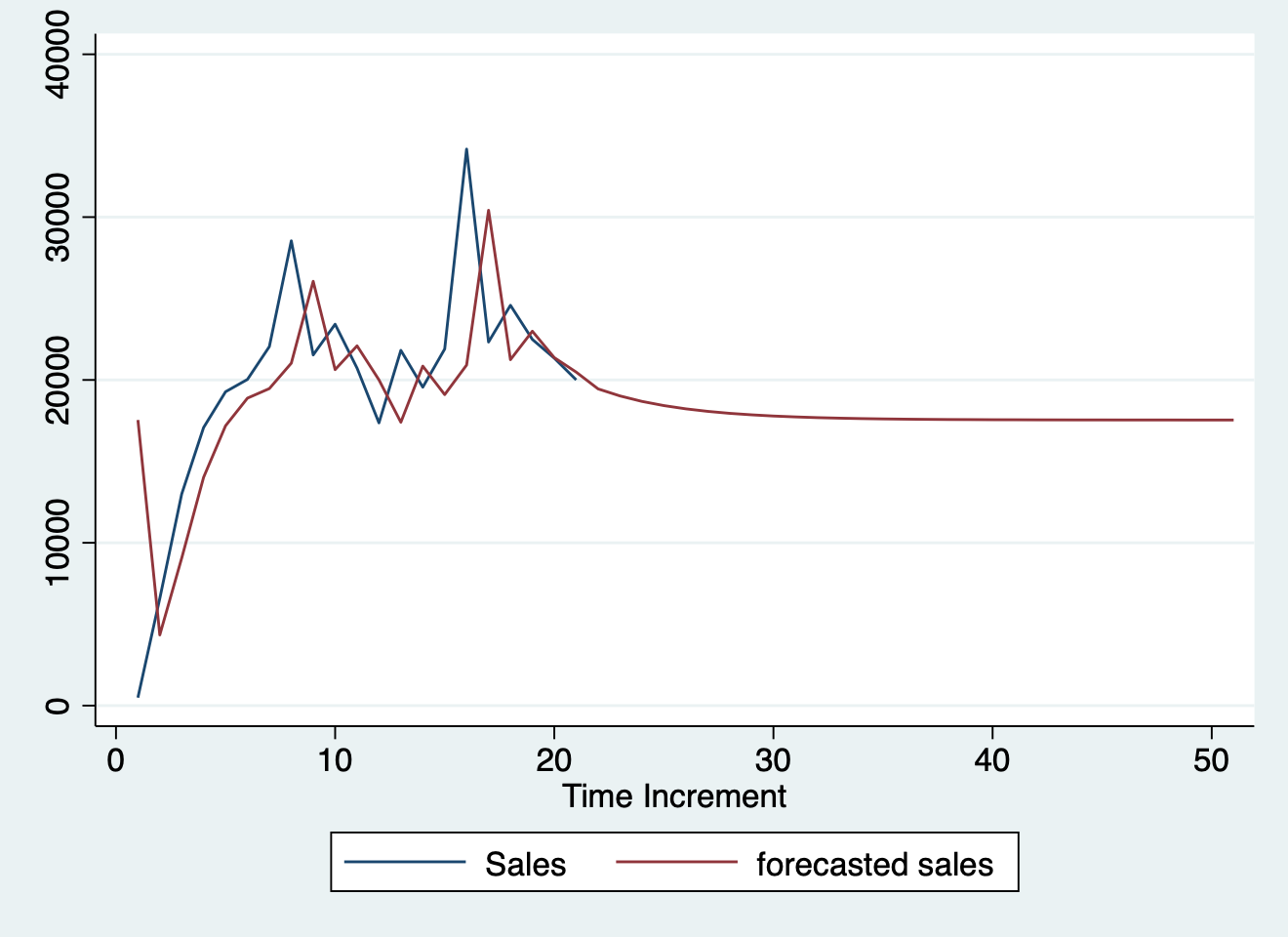
Python
from pandas import DataFrame
#> ModuleNotFoundError: No module named 'pandas'
import statsmodels.api as sm
#> ModuleNotFoundError: No module named 'statsmodels'
import matplotlib as plot
#> ModuleNotFoundError: No module named 'matplotlib'

Stock_Market = {'Year': [2017,2017,2017,2017,2017,
                         2017,2017,2017,2017,2017,
                         2017,2017,2016,2016,2016,
                         2016,2016,2016,2016,2016,
                         2016,2016,2016,2016],
                'Month': [12, 11,10,9,8,7,6,5,4,
                          3,2,1,12,11,10,9,8,7,6,
                          5,4,3,2,1],
                'Interest_Rate':[2.75,2.5,2.5,2.5,2.5,2.5,
                                 2.5,2.25,2.25,2.25,2,2,2,1.75,1.75,
                                 1.75,1.75,1.75,1.75,1.75,1.75,1.75,1.75,1.75],
                'Unemployment_Rate':[5.3,5.3,5.3,5.3,5.4,5.6,
                                     5.5,5.5,5.5,5.6,5.7,5.9,6,5.9,5.8,6.1,
                                     6.2,6.1,6.1,6.1,5.9,6.2,6.2,6.1],
                'Stock_Index_Price': [1464,1394,1357,1293,1256,1254,1234,1195,1159,1167,1130,
                                      1075,1047,965,943,958,971,949,884,866,876,822,704,719]
                }

df = DataFrame(Stock_Market,columns=['Year','Month','Interest_Rate',
                                     'Unemployment_Rate','Stock_Index_Price'])
#> NameError: name 'DataFrame' is not defined

X = df[['Interest_Rate','Unemployment_Rate']]
#> NameError: name 'df' is not defined

# here we have 2 variables for the multiple linear regression. If you just want to use one variable for simple linear regression, then use X = df['Interest_Rate'] for example

Y = df['Stock_Index_Price']
#> NameError: name 'df' is not defined

X = sm.add_constant(X) # adding a constant
#> NameError: name 'sm' is not defined

model = sm.OLS(Y, X).fit()
#> NameError: name 'sm' is not defined
predictions = model.predict(X)
#> NameError: name 'model' is not defined

print_model = model.summary()
#> NameError: name 'model' is not defined
print(print_model)
#> NameError: name 'print_model' is not defined
R
fit <- glm(mpg ~ cyl + disp, mtcars, family = gaussian())
# show the theoretical model
equatiomatic::extract_eq(fit)
E( \operatorname{mpg} ) = \alpha + \beta_{1}(\operatorname{cyl}) + \beta_{2}(\operatorname{disp})
Stata
sysuse auto2, clear
parallel initialize 8, f
mfp: glm price mpg
twoway (fpfitci price mpg, estcmd(glm) fcolor(dkorange%20) alcolor(%40))  || scatter price mpg, mcolor(dkorange) scale(0.75)
graph export "mfp.png", replace
#> . sysuse auto2, clear
#> (1978 automobile data)
#>
#> . parallel initialize 8, f
#> -initialize- invalid parallel subcommand (help parallel)
#> r(198);
#>
#> r(198);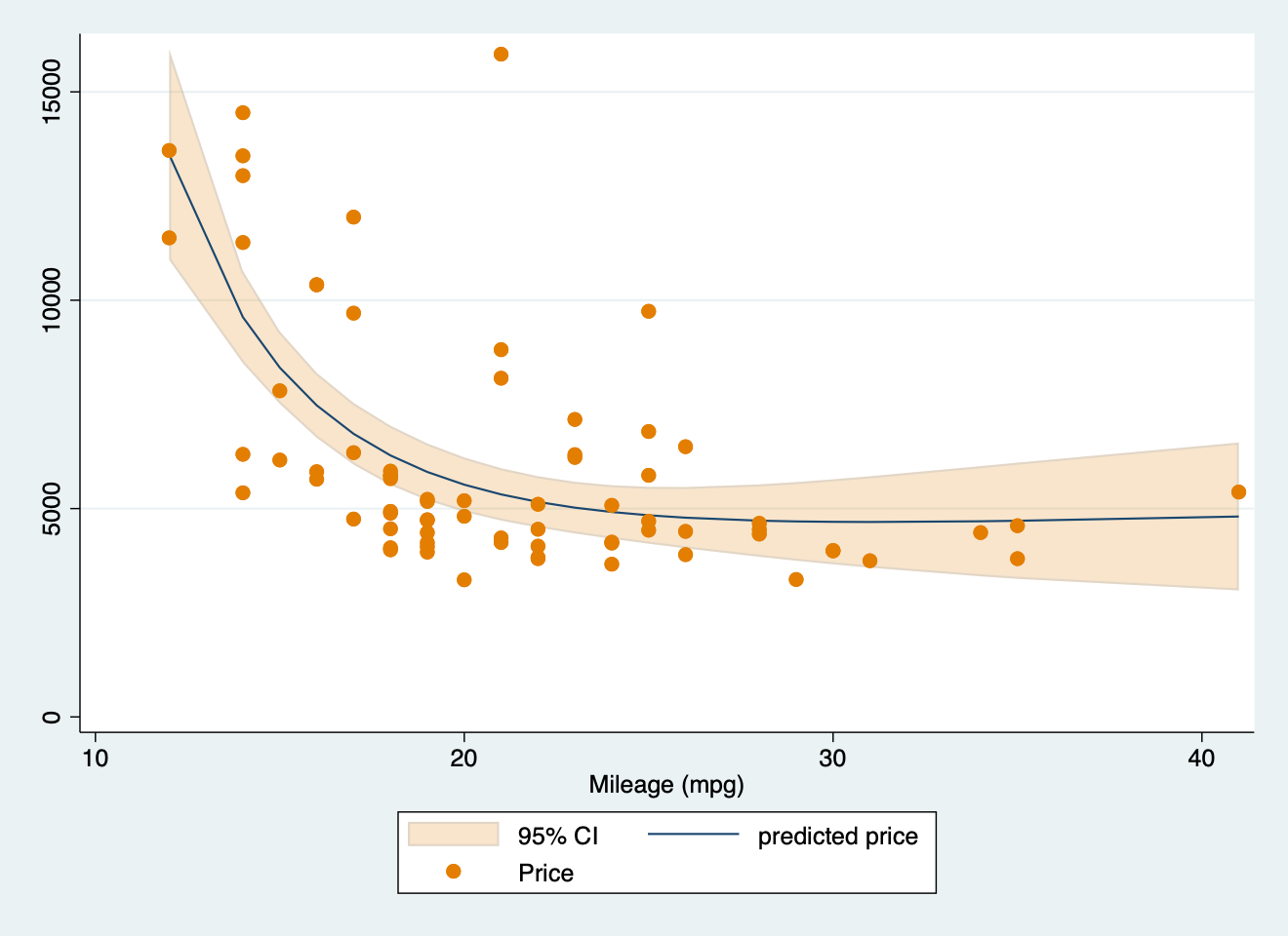
clear
set obs 100
/**
Generate variables from a normal distribution like before
*/
generate x = rnormal(0, 1)
generate y = rnormal(0, 1)
/**
We set up our model here

*/
parallel initialize 8, f
bayesmh y x, likelihood(normal({var})) prior({var}, normal(0, 10)) ///
prior({y:}, normal(0, 10)) rseed(1031) saving(coutput_pred, replace) mcmcsize(1000)
/**
We use the bayespredict command to make predictions from the model
*/
bayespredict (mean:@mean({_resid})) (var:@variance({_resid})), ///
rseed(1031) saving(coutput_pred, replace)
/**
Then we calculate the posterior predictive P-values
*/
bayesstats ppvalues {mean} using coutput_pred
#> . clear
#>
#> . set obs 100
#> Number of observations (_N) was 0, now 100.
#>
#> . /**
#> > Generate variables from a normal distribution like before
#> > */
#> . generate x = rnormal(0, 1)
#>
#> . generate y = rnormal(0, 1)
#>
#> . /**
#> > We set up our model here
#> >
#> > */
#> . parallel initialize 8, f
#> -initialize- invalid parallel subcommand (help parallel)
#> r(198);
#>
#> r(198);library(lme4)
library(simr)
# Toy model
fm = lmer(y ~ x + (x | g), data = simdata)
# Extend sample size of `g`
fm_extended_g = extend(fm, along = 'g', n = 4)
# 4 levels of g
pwcurve_4g = powerCurve(fm_extended_g, fixed('x'), along = 'g', breaks = 4,
nsim = 50, seed = 123,
# No progress bar
progress = FALSE)
# 6 levels of g
# Create a destination object using any of the power curves above.
all_pwcurve = pwcurve_4g
# Combine results
all_pwcurve$ps = c(pwcurve_4g$ps[1])
# Combine the different numbers of levels.
all_pwcurve$xval = c(pwcurve_4g$nlevels)
print(all_pwcurve)
#> Power for predictor 'x', (95% confidence interval),
#> by number of levels in g:
#> 4: 44.00% (29.99, 58.75) - 40 rows
#>
#> Time elapsed: 0 h 0 m 4 s
plot(all_pwcurve, xlab = 'Levels of g')
https://www.datacamp.com/datalab/w/2c40d510-1d81-4078-8ae3-9dcdd8f2a21b/edit#welcome-environment
https://www.datacamp.com/datalab/w/bf3f12b6-9b15-400f-8f0e-674b33b29cbe/print-report/notebook.ipynb#1-load-your-datahttps://www.datacamp.com/datalab/w/2c40d510-1d81-4078-8ae3-9dcdd8f2a21b/edit#considered-exemption

Citation
BibTeX citation:
@misc{panda2018,
  author = {Panda, Sir},
  title = {Stan: {Bayesian} {Modeling} {Examples}},
  date = {2018-01-01},
  url = {https://lesslikely.com/posts/statistics/stan},
  langid = {en},
  abstract = {Sample scripts and examples for Bayesian modeling using
    Stan.}
}
For attribution, please cite this work as:
1. Panda S. (2018). ‘Stan: Bayesian Modeling Examples’.
Less Likely. https://lesslikely.com/posts/statistics/stan.