

Around April of last year, a group of surgeons published a paper in the Annals of Surgery (apparently one of the most read journals in surgical science) where they suggested that CONSORT and STROBE guidelines be modified to recommend calculations of post-hoc power, specifically observed power.
They write,
“But, as 80% power is difficult to achieve in surgical studies, we argue that the CONSORT and STROBE guidelines should be modified to include the disclosure of power—even if less than 80%—with the given sample size and effect size observed in that study.”
Some folks noticed, including Andrew Gelman, who decided to write a letter to the editor (LTE) explaining why this is a bad idea.
Gelman writes in the LTE,
“This would be a bad idea. The problem is that the (estimated) effect size observed in a study is noisy, especially so in the sorts of studies discussed by the authors. Using estimated effect size can give a terrible estimate of power, and in many cases can lead to drastic overestimates of power (thus, extreme overconfidence of the sort that is rightly deplored by Bababekov et al. in their article), with the problem becoming even worse for studies that happen to achieve statistical significance.
The problem is well known in the statistical and medical literatures; see, e.g., Lane and Dunlap (1978), Hedges (1984), Goodman and Berlin (1994), Senn (2002), and Lenth (2007). For some discussion of the systemic consequences of biased power calculations based on noisy estimates of effect size, see Button et al. (2013), and for an alternative approach to design and power analysis, see Gelman and Carlin (2014).”
“We Respectfully Disagree”
The authors replied of course, where most of their argument boils down to,
“We respectfully disagree that it is wrong to report post hoc power in the surgical literature. We fully understand that P value and post hoc power based on observed effect size are mathematically redundant; however, we would point out that being redundant is not the same as being incorrect… We also respectfully disagree that knowing the power after the fact is not useful in surgical science.”
Andrew Gelman notices and happens to blog about it, and also gets a chance to write a response to the response to the response to the original paper.
Guess now it’s over. Or well… we thought!
Zombie Power
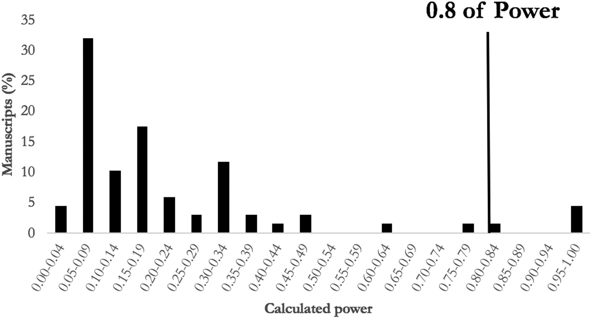
Same group of surgeons come back with a completely new paper where they conducted a review of the surgical literature, removed all significant results, and calculated the observed power of each nonsignificant study.
They summarize their findings,
“In this analysis of the current, high-impact surgical literature, we found the median power in studies concluding insignificant differences was 0.16, with only four studies reaching the standard of 0.8.”
They also draw some interesting parallels in their discussion section to show how change can be difficult but necessary,
“The continued inability of surgical studies to reach power of 0.8 should raise the following salient questions: Are we aiming for an arbitrary standard that can rarely be achieved? Are we discrediting the academic contributions of studies that do not reach the arbitrary 0.8 threshold? And, should we reconsider the power standard in surgical science so that it is more applicable to surgery?
It is not unreasonable to challenge standards that may not be applicable. Before 1971, the voting age was arbitrarily set at 21 years old in the United States. The 26th Amendment lowered the voting age to 18 years in 1971 to acknowledge the contributions of all military servicemen and women, many of whom were under age 21 years and could not vote under earlier laws. Similarly, the surgical community should reconsider the arbitrary power threshold to recognize the contribution of studies in the surgical literature that have been arbitrarily discounted as underpowered.
The Frustration & Wrath of Statisticians
The statistical community noticed once again, and this led to a explosion on Twitter, DataMethods, and PubPeer.
I also happened to write something (found below, which I also posted on DataMethods and PubPeer) and constructed some simulations to argue why the authors are promoting something misleading.
My Response
Despite statisticians warning against the use of observed power for decades (Hoenig & Heisey, 2001), the practice continues, usually from research groups who are unaware of the problems with it. Bababekov et al. (the authors of this paper) have not only defended their use of observed power in previous papers, even when criticized by statisticians who have looked into the problem, but unfortunately, they encourage others in surgical science to do the same.
The arguments put forth in this paper have no mathematical or empirical basis. Meaning, Bababekov et al. have not given any mathematical proofs or simulated data to make their case. Their argument merely consists of,
“Although it has been argued that P value and post hoc power based on observed effect size are mathematically redundant; we assert that being redundant is not the same as being incorrect.”
“We believe this redundancy is necessary in the unique case of surgical science, as post hoc power improves the communication of results by supplementing information provided by the P value.(12) Moreover, post hoc power provides a single metric to help readers better appreciate the limitation of a study.”
The problem is that this practice is not only redundant, it is
incorrect and highly misleading. This can easily be shown with
simulated data (see images below). Here, I simulate
Group A has a mean of
In this simulation, the studies can be categorized by nine different
sample sizes, meaning they have varying true power (something we know
because it’s a simulation). True power ranges all the way from
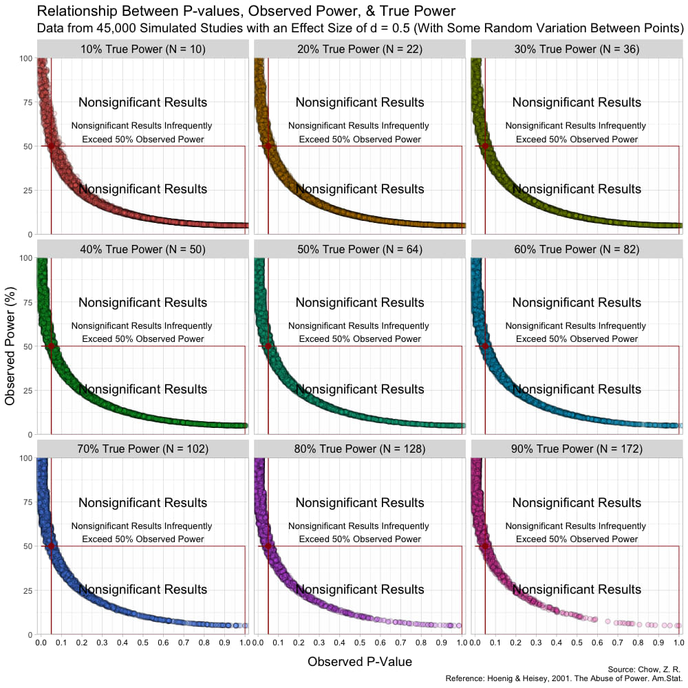
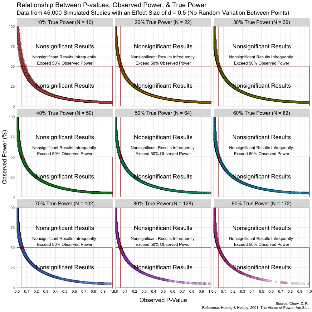
The graph above has some random variation added between points to make them out, but in reality, this (below) is what the graph looks like without any random variation at all. (These are not lines, but actual points plotted!)
In animated form:
Notice that despite true power being known for each of these studies,
observed power highly varies within these scenarios, especially for
studies with low(er) power. For example, when true power is set at
This is because Babakev et al. does not seem to understand long-term
frequencies. Statistical power is a frequentist concept, meaning that if
someone designs a study with the hope of the test correctly detecting a
dimensional violation by the test hypothesis (such as the null
hypothesis)
This does not mean that the study itself has an
Furthermore, because the P-value is a random variable and measures random error in the estimate (Greenland, 2019), taking it (observed P) from a single study and transforming it into a distorted version of power (observed power) is beyond fallacious. The authors not only confuse observed power and true power, but they also confuse the random variable P with its realization, observed P. Observed P-values are useful because they indicate statistical compatibility between the observed data and the test hypothesis.
If they are being used for decision rules with a set alpha, and the researchers suspect that a type-II error was very likely, they can use the computed confidence / compatibility / consonance intervals to see what effect sizes are within the interval and how wide the interval estimates are (which measure random error/precision).
However, Bababekov et al. does not see this as a solution as they argue here,
“An alternative solution to mitigate risk of misinterpreting P > 0.05 is for surgical investigators to report the confidence intervals in their results along with the P value.”
“However, the general audience would likely pay more attention to the overlap of confidence intervals in a comparative study with two or more comparison groups with multiple confidence intervals, and still misinterpret the findings as demonstrating equivalency.”
The problem here is that investigators confusing overlapping intervals for equivalency is a cognitive problem (Greenland, 2017) where they do not understand what frequentist intervals are rather than a defect in the method itself.
A computed frequentist interval, such as a
Thus, it is largely irrelevant whether two or more confidence/consonance intervals overlap. The useful questions are:
- how wide are these intervals?
- how much do they overlap?
- what effect sizes do they span?
Better than computing a single interval estimate for a particular alpha
level is to compute the
function,
where every interval estimate is plotted with its corresponding alpha
(
Bababekov et al. instead sees observed power as being a solution to the “problems” they highlight with interval estimates,
“Power provides a single metric to help readers better appreciate the limitation of a study. As such, we believe reporting power is the most reasonable solution to avoid misinterpreting P > 0.05.”
This argument further highlights the problems with trying to come to conclusions from single studies. The authors wish to answer
“Was my study large enough and reliable, and if not, what single metric can I use to better understand how reliable the decision (reject/fail to reject) is?”
For this, they have found a method, one that they reify, that helps to address their uncertainties of the data-generation process, but unfortunately, it is unreliable and cannot do what they wish it does.
As others have pointed out above, the arguments put forth in this paper are fallacious and thus the manuscript itself is defective and has the potential to seriously mislead many surgical investigators who are not well versed in statistical methods. Letters to the editor (of which there are numerous) and corrections are simply not enough. A retraction is necessary when a manuscript is this defective.
Script to Reproduce Simulations
Also, the R code to reproduce the simulations:
First, we load the necessary R packages to do so.
library("pwr")
library("ggplot2")#' @title Simulate Retrospective Power
#' @param N
#' @param MeanA
#' @param MeanB
#' @param SD
#' @param pwr
#' @return
#' @export
#' @examples
falsepower <- function(N, MeanA, MeanB, SD, pwr) {
# Generates random values from a normal distribution.
x <- rnorm(N, MeanA, SD)
y <- rnorm(N, MeanB, SD)
# runs a statistical test between the two groups above and
# extracts the observed P-values and stores in an object
pvalues <- t.test(x, y)$p.value
# Computes the standard deviations of both groups and pools them and stores it
pooledsd <- sqrt((((N - 1)) * (sd(x)^2) +
((N - 1) * (sd(y)^2)))
/ ((N * 2) - 2))
# Calculate the standardized, observed effect size
obses <- abs(mean(x) - mean(y)) / pooledsd
# Calculates the observed power using the observed effect size
obspower <- pwr.t.test(N, obses, sig.level = 0.05, type = "two.sample",
alternative = "two.sided")$power
df <- data.frame(pvalues, obspower)
df$pvalues <- round(df$pvalues, digits = 2)
df$obspower <- round((df$obspower * 100), digits = 2)
df$truepower <- pwr
return(df)
}
# Here, we produce 9 different scenarios where know the
# the assumed power and calculate observed
# Edit the values here if you wish to set
# different means, standard deviations, or sample sizes
df10 <- do.call("rbind", replicate(5000, (falsepower(N = 5,
MeanA = 25, MeanB = 20, SD = 10,
pwr = "10% True Power (N = 10)")),
simplify = FALSE))
df20 <- do.call("rbind", replicate(5000, (falsepower(N = 11,
MeanA = 25, MeanB = 20, SD = 10,
pwr ="20% True Power (N = 22)")),
simplify = FALSE))
df30 <- do.call("rbind", replicate(5000, (falsepower(N = 18,
MeanA = 25, MeanB = 20, SD = 10,
pwr = "30% True Power (N = 36)")),
simplify = FALSE))
df40 <- do.call("rbind", replicate(5000, (falsepower(N = 25,
MeanA = 25, MeanB = 20, SD = 10,
pwr = "40% True Power (N = 50)")),
simplify = FALSE))
df50 <- do.call("rbind", replicate(5000, (falsepower(N = 32,
MeanA = 25, MeanB = 20, SD = 10,
pwr = "50% True Power (N = 64)")),
simplify = FALSE))
df60 <- do.call("rbind", replicate(5000, (falsepower(N = 41,
MeanA = 25, MeanB = 20, SD = 10,
pwr = "60% True Power (N = 82)")),
simplify = FALSE))
df70 <- do.call("rbind", replicate(5000, (falsepower(N = 51,
MeanA = 25, MeanB = 20, SD = 10,
pwr = "70% True Power (N = 102)")),
simplify = FALSE))
df80 <- do.call("rbind", replicate(5000, (falsepower(N = 64,
MeanA = 25, MeanB = 20, SD = 10,
pwr = "80% True Power (N = 128)")),
simplify = FALSE))
df90 <- do.call("rbind", replicate(5000, (falsepower(N = 86,
MeanA = 25, MeanB = 20, SD = 10,
pwr = "90% True Power (N = 172)")),
simplify = FALSE))
# Combine the dataframes
df <- rbind(df10, df20, df30, df40, df50, df60, df70, df80, df90)
# Graph the data with facets
ggplot(data = df, mapping = aes(x = pvalues, y = obspower)) +
geom_jitter(aes(fill = truepower), alpha = 0.2,
shape = 21, stroke = 0.7, size = 2) +
annotate("rect", xmin = 0.05, xmax = 1,
ymin = 0, ymax = 50, color = "#990000",
alpha = .005, size = 0.3) +
annotate("pointrange", x = 0.05, y = 50, ymin = 0, ymax = 100,
colour = "#990000", alpha = 0.8, size = .5) +
annotate("segment", x = 0, xend = 0.05, y = 50, yend = 50,
colour = "#990000") +
annotate(geom = "text", x = 0.5, y = 58,
label = "Nonsignificant Results Infrequently \nExceed 50% Observed Power",
size = 3.5, color = "#000000") +
annotate(geom = "text", x = 0.5, y = 26,
label = "Nonsignificant Results", size = 5, color = "#000000") +
annotate(geom = "text", x = 0.5, y = 75,
label = "Nonsignificant Results", size = 5, color = "#000000") +
facet_wrap( ~ truepower, ncol = 3) +
labs(title = "Relationship Between P-values, Observed Power, & True Power",
subtitle = "Data from 45,000 Simulated Studies with an Effect Size of
d = 0.5 (No Random Variation Between Points)",
x = "Observed P-Value",
y = "Observed Power (%)",
fill = "True Power") +
theme_light() +
theme(legend.position = "none",
axis.title.x = element_text(size = 14, vjust = -2),
axis.text.x = element_text(color = '#000000'),
axis.title.y = element_text(size = 14),
strip.background = element_rect(fill = "#dddddd" ),
strip.text = element_text(color = 'black', size = 12)) +
scale_x_continuous(breaks = seq(0, 1, .10), expand = c(0, 0)) +
scale_y_continuous(breaks = seq(0, 100, 25), expand = c(0, 0)) +
theme(text = element_text(color = "#000000")) +
theme(plot.title = element_text(size = 16),
plot.subtitle = element_text(size = 14))
Environment
The analyses were run on
#> R version 4.4.3 (2025-02-28)
#> Platform: aarch64-apple-darwin20
#> Running under: macOS Sequoia 15.4
#>
#> Matrix products: default
#> BLAS:   /Library/Frameworks/R.framework/Versions/4.4-arm64/Resources/lib/libRblas.0.dylib
#> LAPACK: /Library/Frameworks/R.framework/Versions/4.4-arm64/Resources/lib/libRlapack.dylib;  LAPACK version 3.12.0
#>
#> Random number generation:
#>  RNG:     Mersenne-Twister
#>  Normal:  Inversion
#>  Sample:  Rejection
#>
#> locale:
#> [1] en_US.UTF-8/en_US.UTF-8/en_US.UTF-8/C/en_US.UTF-8/en_US.UTF-8
#>
#> time zone: America/New_York
#> tzcode source: internal
#>
#> attached base packages:
#>  [1] splines   grid      stats4    parallel  stats     graphics  grDevices utils     datasets  methods   base
#>
#> other attached packages:
#>  [1] pwr_1.3-0             texPreview_2.1.0      tinytex_0.56          rmarkdown_2.29        brms_2.22.0
#>  [6] bootImpute_1.2.2      knitr_1.50            boot_1.3-31           JuliaCall_0.17.6      reshape2_1.4.4
#> [11] ProfileLikelihood_1.3 ImputeRobust_1.3-1    gamlss_5.4-22         gamlss.dist_6.1-1     gamlss.data_6.0-6
#> [16] mvtnorm_1.3-3         performance_0.13.0    summarytools_1.1.3    tidybayes_3.0.7       htmltools_0.5.8.1
#> [21] Statamarkdown_0.9.2   car_3.1-3             carData_3.0-5         qqplotr_0.0.6         ggcorrplot_0.1.4.1
#> [26] mitml_0.4-5           pbmcapply_1.5.1       Amelia_1.8.3          Rcpp_1.0.14           blogdown_1.21.1
#> [31] doParallel_1.0.17     iterators_1.0.14      foreach_1.5.2         lattice_0.22-7        bayesplot_1.12.0
#> [36] wesanderson_0.3.7     VIM_6.2.2             colorspace_2.1-1      here_1.0.1            progress_1.2.3
#> [41] loo_2.8.0             mi_1.1                Matrix_1.7-3          broom_1.0.8           yardstick_1.3.2
#> [46] svglite_2.1.3         Cairo_1.6-2           cowplot_1.1.3         mgcv_1.9-3            nlme_3.1-168
#> [51] xfun_0.52             broom.mixed_0.2.9.6   reticulate_1.42.0     kableExtra_1.4.0      posterior_1.6.1
#> [56] checkmate_2.3.2       parallelly_1.43.0     miceFast_0.8.5        randomForest_4.7-1.2  missForest_1.5
#> [61] miceadds_3.17-44      quantreg_6.1          SparseM_1.84-2        MCMCpack_1.7-1        MASS_7.3-65
#> [66] coda_0.19-4.1         latex2exp_0.9.6       rstan_2.32.7          StanHeaders_2.32.10   lubridate_1.9.4
#> [71] forcats_1.0.0         stringr_1.5.1         dplyr_1.1.4           purrr_1.0.4           readr_2.1.5
#> [76] tibble_3.2.1          ggplot2_3.5.2         tidyverse_2.0.0       ggtext_0.1.2          concurve_2.8.0
#> [81] showtext_0.9-7        showtextdb_3.0        sysfonts_0.8.9        future.apply_1.11.3   future_1.40.0
#> [86] tidyr_1.3.1           magrittr_2.0.3        mice_3.17.0           rms_8.0-0             Hmisc_5.2-3
#>
#> loaded via a namespace (and not attached):
#>   [1] nnet_7.3-20             TH.data_1.1-3           vctrs_0.6.5             digest_0.6.37           png_0.1-8
#>   [6] shape_1.4.6.1           proxy_0.4-27            magick_2.8.6            fontLiberation_0.1.0    withr_3.0.2
#>  [11] ggpubr_0.6.0            survival_3.8-3          doRNG_1.8.6.2           emmeans_1.11.0          MatrixModels_0.5-4
#>  [16] systemfonts_1.2.2       ragg_1.4.0              zoo_1.8-14              V8_6.0.3                ggdist_3.3.2
#>  [21] DEoptimR_1.1-3-1        Formula_1.2-5           prettyunits_1.2.0       rematch2_2.1.2          httr_1.4.7
#>  [26] rstatix_0.7.2           globals_0.16.3          rstudioapi_0.17.1       extremevalues_2.4.1     pan_1.9
#>  [31] generics_0.1.3          base64enc_0.1-3         curl_6.2.2              mitools_2.4             desc_1.4.3
#>  [36] xtable_1.8-4            svUnit_1.0.6            pracma_2.4.4            evaluate_1.0.3          hms_1.1.3
#>  [41] glmnet_4.1-8            bookdown_0.42           lmtest_0.9-40           robustbase_0.99-4-1     matrixStats_1.5.0
#>  [46] svgPanZoom_0.3.4        class_7.3-23            pillar_1.10.2           caTools_1.18.3          compiler_4.4.3
#>  [51] stringi_1.8.7           jomo_2.7-6              minqa_1.2.8             plyr_1.8.9              crayon_1.5.3
#>  [56] abind_1.4-8             metadat_1.4-0           sp_2.2-0                mathjaxr_1.6-0          rapportools_1.2
#>  [61] twosamples_2.0.1        sandwich_3.1-1          whisker_0.4.1           codetools_0.2-20        multcomp_1.4-28
#>  [66] textshaping_1.0.0       bcaboot_0.2-3           openssl_2.3.2           flextable_0.9.7         bslib_0.9.0
#>  [71] QuickJSR_1.7.0          e1071_1.7-16            gridtext_0.1.5          lme4_1.1-37             fs_1.6.5
#>  [76] itertools_0.1-3         listenv_0.9.1           Rdpack_2.6.4            pkgbuild_1.4.7          estimability_1.5.1
#>  [81] ggsignif_0.6.4          tzdb_0.5.0              pkgconfig_2.0.3         tools_4.4.3             cachem_1.1.0
#>  [86] rbibutils_2.3           viridisLite_0.4.2       DBI_1.2.3               numDeriv_2016.8-1.1     fastmap_1.2.0
#>  [91] scales_1.3.0            sass_0.4.9              officer_0.6.8           opdisDownsampling_1.0.1 insight_1.1.0
#>  [96] rpart_4.1.24            reformulas_0.4.0        survminer_0.5.0         yaml_2.3.10             foreign_0.8-90
#> [ reached getOption("max.print") -- omitted 53 entries ]Help support the website!
