Book Review: Fisher, Neyman, and the Creation of Classical Statistics
classical statistics, egon pearson, fisher, inverse probability, neyman and fisher, statistical methods for research workers
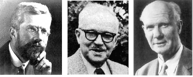
Erich Lehmann’s last book,1 which was published after his death, is on the history of classical statistics and its creators. Specifically, how his mentor Jerzy Neyman and his adversary Ronald Fisher helped lay the foundations for the methods that are used today in several fields.
A Very Brief History of Classical Statistics
This post is intended to be a general review/summary of the book, which I recommend to everyone and anyone who is interested in statistics and science. The book clears up several misconceptions people have about how frequentist statistics came to be the dominant school of statistics. Thus, I want to go over four topics from Lehmann’s book that I believe people should know more about:
How the founders of classical statistics viewed Bayesian inference
What they each developed
How they came to become so conflicted
And how their views changed over time
Where Are The Bayesians?
As Stephen Senn points out in his Fisher Memorial Lecture at the Royal Statistical Society, there is a common myth that everyone who practiced applied statistics before the early 20th century was using Bayesian inference and doing everything correctly, but then Fisher came in and created significance testing, thus giving researchers a powerful tool to easily hack their data and produce publishable results, and now we have several replication crises because of this.
Of course, this is far from the truth and any thorough investigation into the history of statistics will clear up this up amongst many other misconceptions.
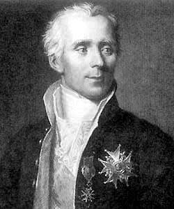
As several individuals may know, it was Thomas Bayes who came up with Bayes theorem and it was Richard Price who disseminated most of his writings after Bayes’s death. However, as many self-identified Bayesians will attest, using Bayes’ theorem does not make one a Bayesian. It is actually quite hard to know how Bayes would react to modern Bayesian inference. The Bayesian inference that we are familiar with today can be attributed to Pierre-Simon Laplace, who popularized what is now known as “objective Bayes.”
Back then, it was not called “Bayesian inference” but was referred to as “inverse probability” and it was a method used by many before the dominance of classical statistics. So this is one part that common myths get right. Inverse probability did indeed have a moment in history before the dominance of frequentist statistics.
Laplace, and several others popularized such methods, but around the end of the 19th century, the tides began to shift. Several mathematicians and statisticians began to discourage the use of inverse probability because they saw it as a nonrigorous method of data analysis.
This can be seen in the following passages about Fisher.
“His first publication on this new approach to inference was a 1930 paper “Inverse probability.” The paper begins with a critique of the inverse (Bayesian) method. This section ends with Fisher’s asking:
If, then, we follow writers like Boole, Venn and Chrystal in rejecting the inverse argument as devoid of foundation and incapable even of consistent application, how are we to avoid the staggering falsity of saying that however extensive our knowledge of the values of x may be, yet we know nothing and can know nothing about the values of ?” (78)
Thus, Fisher was not the first to reject inverse probability, he was building on arguments from proto frequentists who already began to condemn inverse probability. Neyman was also a serious critic of inverse probability. In fact, he was probably more of a critic of it at a later point in time then Fisher (much on that later)!
“On one subject, Fisher and Neyman agreed. Fisher, after 1922, and Neyman, after 1937, were united in their strong opposition to the use of prior distributions (unless they were based on substantial empirical evidence).” (90)
Although the two giants of classical statistics both condemned inverse probability, it withstood their influential criticisms.
“It seems ironic that one of the most significant developments after Fisher and Neyman had established their foundations was to rejuvenate an approach they both had strongly opposed and thought to have vanquished: inverse probability…
The nineteenth century approach to inverse probability, championed particularly by Laplace, considered the prior distribution to represent complete ignorance. This concept, now called objective Bayes, was taken up and improved by the Cambridge geophysicist Harold Jeffreys, culminating in his 1939 book, “Theory of Probability.”
A different Bayesian approach, called subjective, was proposed by Ramsey (1926) and Bruno de Finetti in the 1930s. It considered probability as a measure of a person’s subjective degree of uncertainty about a situation. This view came into its own with the publication in 1954 of L. J. Savage’s book, “Foundations of Statistics,” in which he derives the existence of such subjective probabilities from a few, quite plausible, axioms.” (91)
Now that we have looked at how the founders of classical statistics viewed and attempted to discourage the use of inverse probability, we can move onto a brief summary of each of their individual contributions.
Fisher’s Contributions
Much of Fisher’s early work was a result of two individuals, Karl Pearson and William Gosset. Pearson’s work on the method of moments to estimate parameters led to Fisher developing his superior estimation method, maximum likelihood, which he presented in his 1922 foundations paper, “On the mathematical foundations of theoretical statistics.”
“Having defined the problem of statistics to be the estimation of parameters, Fisher states the properties that he desires for his estimators. They are consistency, efficiency, and sufficiency…
He then proposes what he had already suggested earlier in the section on the solution of the estimation problem, the method of maximum likelihood, which “consists, then, simply of choosing such values of these parameters as have the maximum likelihood.” Fisher believes that this method satisfies his three criteria, in particular that it satisfied the criterion of sufficiency, although he states that he “is not satisfied as to the mathematical rigor of any proof which I can put forward to that effect.” He also claims that sufficiency implies efficiency…
Thus, in this paper Fisher has not only formulated the general problem of optimal estimation, but he has also provided a solution. It is a stunning achievement.” (10)
Gosset’s initial work on test statistics, his inability derive proofs for small sample methods, and constant prodding led to Fisher developing several statistical tests which ended up being published in his highly influential book, Statistical Methods For Research Workers,
“For testing the value of a population mean, it had been customary to use a statistic equivalent to what today is called Student’s t, and to refer to the normal distribution. For large samples, this provided a good approximation.
However, Gosset soon realized that for the small samples with which he had to work, the approximation was inadequate. He then had the crucial insight that exact results could be obtained by making an additional assumption, namely that the form of the distribution of the observations is known. Gosset undertook to determine it for the case that the underlying distribution is normal, and he obtained the correct result, although he was not able to give a rigorous proof.
The first proof was obtained (although not published) by Fisher in 1912. His proof was finally published in 1915 [4], together with the corresponding proof for the correlation coefficient that Student had conjectured in a second paper of 1908(b). Fisher followed this in 1921 [14] with a derivation of the distribution of the intraclass correlation coefficient. And then, as a result of constant prodding and urging by Gosset, he found a number of additional small-sample distributions, and in 1925 presented the totality of these results in his book, “Statistical Methods for Research Workers.” (6)
In the book, Fisher’s main focus was on statistical testing and not estimation, and he made this clear,
“…the prime object of this book is to put into the hands of research workers… the means of applying statistical tests accurately to numerical data accumulated in their own laboratories … and later refers to the exact distributions with the use of which this book is chiefly concerned… Thus, the book does not primarily deal with estimation but with significance testing. In fact, estimation is never again mentioned.” (16)
His section about chi-squared tests and significance testing became highly influential,
“In preparing this table we have borne in mind that in practice we do not want to know the exact value of P for any observed , but, in the first place, whether or not the observed value is open to suspicion. If P is between .1 and .9 there is certainly no reason to suspect the hypothesis tested. If it is below .02 it is strongly indicated that the hypothesis fails to account for the whole of the facts. We shall not often be astray if we draw a conventional line at .05 and consider that higher values of indicate a real discrepancy.” (17)
He also presents examples,
“In the first of these, in particular, he finds a p-value between 0.01 and 0.02 and concludes: “If we take P = 0.05 as the limit of significant deviation, we shall say that in this case the deviations from expectation are significant.” (17)
And he expanded on significance testing with analysis of variance, which he had derived while working at Rothamsted analyzing crop data. The book was a large success,
“The first edition of 1,050 copies was sold out after three years, and the second edition of 1,250 copies in another two. Every two to three years necessitated a new edition, which usually contained some improvements and often additions. The size of the editions steadily increased and the eleventh edition of 1950 ran to 7,500 copies. The last edition, the fourteenth, was published posthumously in 1970 from notes Fisher had prepared before his death in 1962.” (25)
And set the groundwork for his next task, discussing experimental methods, which would be published in his second book, The Design of Experiments. In it, he discusses how techniques like randomization were necessary for the validity of statistical tests and how they perform amongst a wide variety of distributions,
“Randomisation properly carried out … ensures that the estimates of error will take proper care of all such causes of different growth rates, and relieves the experimenter from the anxiety of considering and estimating the magnitude of the innumerable causes by which his data may be disturbed. The one flaw in Darwin’s procedure was the absence of randomisation…
It seems to have escaped recognition that the physical act of randomisation which, as has been shown, is necessary for the validity of any test of significance, affords the means, in respect of any particular body of data, of examining the wider hypothesis in which no normality of distribution is implied.” (66)
Although he had proposed randomization tests as a way of dealing with nonnormal distributions, due to their tedious calculations, they never became popular at the time. The book also touched on several other concepts such as randomized blocks, Latin squares, and factorial designs. He also made his position very clear on significance tests and the null hypothesis,
“By increasing the size of the experiment, we can render it more sensitive, meaning by this that it will allow of the detection of a lower degree of sensory discrimination… . Since in every case the experiment is capable of disproving, but never of proving this hypothesis, we may say that the value of the experiment is increased whenever it permits the null hypothesis to be more readily disproved.” (64)
Here we can see Fisher’s concept of statistical power, though “sensitivity” was never a quantified concept. He also clearly states his position on the null hypothesis, that we can never accept it, a mistake that many researchers continue to make today.
Now that we have discussed some of Fisher’s contributions to classical statistics, we can discuss the contributions of Jerzy Neyman.
Neyman’s Contributions

Just like Fisher, Neyman was also impacted by Gosset. However, the influence was indirect. In the 1920s, Egon Pearson, had come across the small-sample tests that both Fisher and Gosset had popularized and had the realization that he must make a name for himself if he ever wished to be free of his father’s influence.
“In 1925-6, I was in a state of puzzlement, and realized that, if I was to continue an academic career as a mathematical statistician, I must construct for myself what might be termed a statistical philosophy, which would have to combine what I accepted from K. P.’s large- sample tradition with the newer ideas of Fisher.” (7)
Thus, he contacted Gosset about practical usage of the t-test, to which Gosset replied,
“Even if the chance is very small, say .00001, that doesn’t in itself necessarily prove that the sample is not drawn randomly from the population [specified by the hypothesis]; what it does is to show that if there is any alternative hypothesis which will explain the occurrence of the sample with a more reasonable probability, say .05 (such as that it belongs to a different population or that the sample wasn’t random or whatever will do the trick), you will be very much more inclined to consider that the original hypothesis is not true.” (E. S. Pearson, 1939.)
“In his obituary of Gosset, Pearson continues, Gosset’s reply had a tremendous influence on the direction of my subsequent work, for the first paragraph contains the germ of that idea which has formed the basis of all the later joint researches of Neyman and myself. It is the simple suggestion that the only valid reason for rejecting a statistical hypothesis is that some alternative explains the observed events with a greater degree of probability.” (7)
As a result, Pearson decided to collaborate with someone who was not taught by his father, but who also had the mathematical abilities to create a generalizable theorem that he had in mind. Thus, began the collaboration between Neyman and Pearson.
In 1928, they published a paper in Biometrika titled, “On the use and interpretation of certain test criteria,” where they introduced two kinds of errors,
Sometimes,when hypothesis A is rejected, will in fact have been drawn from .
More often, in accepting hypothesis A, will really have been drawn from [some alternative population] . (31)
As Lehmann notes, the paper was a great achievement,
“It introduces the consideration of alternatives, the two kinds of error, and the distinction between simple and composite hypotheses. In addition, of course, it proposes the likelihood ratio test. This test is intuitively appealing, and Neyman and Pearson show that in a number of important cases it leads to very satisfactory solutions. It has become the standard approach to new testing problems.” (34)
But the Neyman-Pearson lemma was still incomplete. It was between the years of 1930 and 1933 that Neyman had several insights into how to improve the theory, which Pearson already had felt satisfied with.
“In the next letter, dated March 8, Neyman suggests that he and Egon must “fix a certain plan, as we have lot of problems already started and then left in the wood.” He lists several such problems, among them: to finish what I have started to do with the variation calculus. You will understand it in a moment.
To reduce for a given level the errors of rejecting a true hypothesis, we may use any test. Now we want to find a test which would 1) reduce the probability of rejecting a true hypothesis to the level and 2) such that the probability of accepting a false hypothesis should be minimum. – We find that if such a test exists, then it is the -test. I am now shure [sic] that in a few days I shall be ready. This will show that the “ principle” is not only a principle but that there are arguments to prove that it is really “the best test.”” (35)
These correspondences led to their 1933 paper,
“On the Problem of the Most Efficient Tests of Statistical Hypotheses.” in which both authors introduce the novel idea of behavioral guidance,
“Without hoping to know whether each separate hypothesis is true or false, we may search for rules to govern our behavior with regard to them, in following which we insure that, in the long run of experience, we shall not be too often wrong.” (36)
As Lehmann notes,
“After outlining the general theory, the paper in the next section deals with the case of simple hypotheses and brings the statement and proof of the basic result, now known as the Neyman-Pearson Fundamental Lemma. It states that for testing a simple hypothesis against a simple alternative, the test that at a given level maximizes the probability of rejection is the likelihood ratio test at that level.” (36)
Lehmann summarizes much of the collaboration with the following,
“The collaboration falls into two quite distinct parts. In the early stages, the important ideas, including in particular that of the likelihood ratio principle, all come from Pearson. In fact, Neyman frequency misunderstands them, and continually tries to interpret them in terms of inverse probability.
On the other hand, Pearson is sold on the likelihood ratio principle, which is intuitively appealing and which seems to give reasonable solutions in the cases on which they try it out. But for Neyman, as he is gradually catching on, intuitive appeal is not enough. If the principle is really as good as it appears to be, there ought to be logical justification.
And then one day in early 1930, he sees the light. Since there are two sources of error, one of which is being controlled, the best test is the one minimizing the other one. And from then on, it is Neyman who has the new ideas and Pearson is the reluctant follower. Neyman formulates, and shortly thereafter proves, the Fundamental Lemma and realizes that in some special cases there exist what they later call uniformly most powerful tests. These turn out to coincide with the likelihood ratio tests.” (39)
The Fallout Between The Creators Of Classical Statistics
The conflict between Neyman and Fisher is well known, however, very few are able to accurately point out what lead to each individual strongly detesting the other.
In fact, early correspondences between Neyman and Fisher showed that they were incredibly friendly towards one another. In 1932, Neyman asked Fisher to review their 1933 paper before they submitted it, to which Fisher replied,
“I should be very much interested to see your paper on “the best tests,” as the whole question of tests of significance seems to me to be of immense philosophical importance, and the work you showed me was surely of great promise. It is quite probable that if the work is submitted to the Royal Society, I might be asked to act as referee, and in that case I shall certainly not refuse.” (45)
Fisher not only read the paper, but read it so carefully that he was able to catch a mathematical error and point it out to Neyman and Pearson before it was published,
“When the paper appeared in 1933, the omission was corrected, and a footnote acknowledged that, “We are indebted to Dr. R. A. Fisher – for kindly calling our attention to the fact that we had originally omitted to refer to this restriction.” (46)
Neyman thanked Fisher for his help,
Neyman: “Pearson writes that you have recommended our paper for publication. Although it maybe considered ridiculous to thank a judge, I have intense feeling of gratefulness, which I hope you will kindly accept…” (57)
Fisher replies, “It was a great pleasure to hear from you again.” (57)
Neyman: “I am often thinking that it would be very useful for me to work with you. Unfortunately, this requires considerable amount of money – without speaking of your consent – of course…” (57)
Fisher answers, “You may be sure of my consent,” and in the next letter, “I like hearing from Poland. Best wishes for a Merry Christmas.” (58)
Unfortunately, their relationship began to degrade after the retirement of Karl Pearson. The department of applied statistics that he was the head of was split into the department of statistics, which would be led by his son Egon, and the department of genetics, where Fisher was appointed as Galton professor. Thus, Fisher, one of the creators of classical statistics, was not allowed to teach statistics, while in the floor downstairs, Egon Pearson (a man that he was surely not fond of) was leading the new statistics department.
This change in tone could be seen by the correspondence between Neyman and Fisher following Fisher’s appointment as Galton professor,
“Dr. Pearson writes me that soon you will be Galton Professor at the University College, London. Very probably this means a general reorganization of the Department of Applied Statistics and possibly new people will be needed. I know that there are many statisticians in England and that many of them would be willing to work under you. But improbable things do happen sometimes and you may have a vacant position in your laboratory. In that case please consider whether I can be of any use.” (58)
Fisher replies,
“Many thanks for your letter of congratulation. You will be interested to hear that the Dept. of Statistics has now been separated officially from the Galton Laboratory. I think Egon Pearson is designated as Reader in Statistics. This arrangement will be much laughed at, but it will be rather a poor joke, I fancy, for both Pearson and myself. I think, however, we will make the best of it.
I shall not lecture on statistics, but probably on “the logic of experimentation,” so that my lectures will not be troubled by students who cannot see through a wire fence. I wish I had a fine place for you, but it will be long before my new department can be given any sort of unity and coherence, and you will be head of a faculty before I shall be able to get much done. If in England, do not fail to see me at University College.” (58)
Of course, there is little doubt that both Karl and Egon Pearson contributed to the fallout between Neyman and Fisher. In 1929, Egon Pearson had submitted a critical review of the second edition of Statistical Methods For Research Workers to Nature,
“There is one criticism, however, which must be made from the statistical point of view. A large number of the tests developed are based…on the assumption that the population sampled is of the “normal” form. That this is the case may be gathered from a careful reading of the text, but the point is not sufficiently emphasized.
It does not appear reasonable to lay stress on the “exactness” of the tests when no means whatever are given of appreciating how rapidly they become inexact as the population sampled diverges from normality. That the tests, for example, connected with the analysis of variance are far more dependent on normality than those involving Student’s z (or t) distribution is almost certain, but no clear indication of the need for caution in their application is given.” (22)
As Lehmann points out, Fisher was deeply offended by this review. Nearly six years later (1935), Neyman encountered a similar reaction when he submitted a paper titled, “Statistical problems in agricultural experimentation” pointing out problems with some of the concepts that Fisher had introduced in his book, The Design of Experiments. Fisher was furious,
“I had hoped that Dr. Neyman’s paper would be on a subject with which the author was fully acquainted, and on which he could speak with authority, as in the case of his address to the Society delivered last summer. Since seeing the paper, I have come to the conclusion that Dr. Neyman had been somewhat unwise in his choice of topics… (59)
Were it not for the persistent effort which Dr. Neyman and Dr. Pearson had made to treat what they speak of as problems of estimation, by means merely of tests of significance, I have no doubt that Dr. Neyman would not have been in any danger of falling into the series of misunderstandings which his paper revealed.” (59)
Correspondences from there on out had become hostile,
“Neyman later (Reid 1982, p. 126) recalls that a week after this meeting, Fisher stopped by his room at University College:
And he said to me that he and I are in the same building… . That, as I know, he had published a book – and that’s Statistical Methods for Research Workers – and he is upstairs from me so he knows something about my lectures – that from time to time I mention his ideas, this and that – and that this would be quite appropriate if I were not here in the College but, say, in California – but if I am going to be at University College, then this is not acceptable to him.
And then I said, “Do you mean that if I am here, I should just lecture using your book?” And then he gave an affirmative answer. And I said, “Sorry, no. I cannot promise that.” And then he said, “Well, if so, then from now on I shall oppose you in all my capacities.”
Reid also reports (p. 124) that, After the Royal Statistical Society meeting of March 28, relations between workers on the two floors of K. P.’s old preserve became openly hostile. One evening, late that spring, Neyman and Pearson returned to their department after dinner to do some work.
Entering, they were startled to find strewn on the floor the wooden models which Neyman had used to illustrate his talk on the relative advantages of randomized blocks and Latin squares. They were regularly kept in a cupboard in the laboratory. Both Neyman and Pearson always believed that the models were removed by Fisher in a fit of anger.” (59)
There Is No One Neyman Nor One Fisher
When Fisher released his first edition of Statistical Methods For Research Workers (SMRW), he recommended 5% or 1% as good choices for significance levels, with the latter being used when a “more stringent requirement was necessary.” Fisher was also not interested in exact P-values as pointed out in the section discussing his contributions.
Many of these views changed as he released later editions of his SMRW and his new book, Statistical Methods for Scientific Inference (SMSI). For example, he no longer recommended a particular level of significance,
“In his late, 1956, book SMSI, Fisher protested that “no scientific worker has a fixed level of significance at which from year to year, and in all circumstances, he rejects hypotheses; he rather gives his mind to each particular case, and his ideas” (52)
In the 13th edition of SMRW he stated,
“The actual value of P obtainable from the table by interpolation indicates the strength of the evidence against the hypothesis. A value of exceeding the 5 per cent. point is seldom to be disregarded.” (52)
Thus, Fisher had changed his mind on the topic.
Neyman too had a significant change of mind during the course of his collaboration with Pearson. At first, he constantly defaulted to inverse probability methods, as noted by Pearson’s letter to him in 1978,
“I have eight letters which you wrote to me during February and March 1929, trying to persuade me to put my name as a joint author. But you had introduced an a priori law of probability…, and I was not willing to start from this basis. True we had given the inverse probability as an alternative approach in our 1928 Part I paper, but I must in 1927-28 still have been ready to concede to your line of thought.
However, by 1929 I had come down firmly to agree with Fisher that prior distributions should not be used, except in cases where they were based on real knowledge, e.g., in some Mendelian problems. You were disappointed, but accepted my decision; after all, the whole mathematical development in the paper was yours.” (42)
Though eventually Neyman abandoned his interest in inverse probability and became a serious critic,
“His conviction of the inapplicability of the inverse method had by then become a fundamental part of his statistical philosophy, from which he never wavered.” (42)
Although this post is mainly fixated on the book by Lehmann, I would like to at least paste this one relevant passage from Hulbert & Lombardi, 2009,2
“In a later philosophical essay, Neyman (1977: 112) recounted their cloud-seeding studies, and labeled P values of 0.09, 0.03, and < 0.01 reported in their earlier paper (Lovasich et al. 1971), as “approximately significant,” “significant,” and “highly significant,” respectively. The dichotomies of the paleoFisherian and Neyman-Pearsonian frameworks were quietly admitted to be less appropriate than more nebulous interpretations — at least in cloud work!
Indeed, Cox (2006a: 43, 195) has noted that “the differences between Fisher and Neyman … were not nearly as great as the asperity of the arguments between them might suggest … [and in] actual practice … Neyman … often reported p-values whereas some of Fisher’s use of tests … was much more dichotomous”!
As we can see from a summary of Lehmann’s book, the individuals who founded classical statistics were skilled and talented individuals who were also complex and had various reasons for doing what they did. I hope this blog post encourages readers to fully dive into Lehmann’s book where he gives a far more detailed account of Fisher and Neyman’s contributions to classical statistics.
References
References
Citation
@online{panda2018,
  author = {Panda, Sir and Rafi, Zad},
  title = {Book {Review:} {Fisher,} {Neyman,} and the {Creation} of
    {Classical} {Statistics}},
  date = {2018-12-30},
  url = {https://lesslikely.com/posts/statistics/classical-lehmann.html},
  langid = {en}
}