
set.seed(1031)

# ---- Part A: normal linear model ----
n <- 200
x <- rnorm(n)
y <- 2 + 0.75*x + rnorm(n, sd = 1.5)
X <- cbind(1, x)

negloglik_normal <- function(theta, y, X) {
  beta <- theta[1:2]; log_sigma <- theta[3]
  -sum(dnorm(y, mean = X %*% beta, sd = exp(log_sigma), log = TRUE))
}

fit <- optim(c(0, 0, 0), negloglik_normal, y = y, X = X, method = "BFGS")
b_ml <- fit$par[2]; sigma_ml <- exp(fit$par[3])

ols <- lm(y ~ x)
sigma_ols_nscaled <- sqrt(sum(residuals(ols)^2) / n)   # ML sigma uses n, not n-k

stopifnot(abs(b_ml - coef(ols)[["x"]]) < 1e-4,
          abs(sigma_ml - sigma_ols_nscaled) < 1e-3)
cat("Part A validation PASSED: optim MLE reproduces lm\n")
#> Part A validation PASSED: optim MLE reproduces lm

# ---- Part B: logistic regression ----
n2 <- 300
x2 <- rnorm(n2)
y2 <- as.numeric(runif(n2) < plogis(-0.4 + 0.9*x2))
X2 <- cbind(1, x2)

negloglik_logit <- function(beta, y, X) {
  xb <- X %*% beta
  sum(log1p(exp(-xb))*y + log1p(exp(xb))*(1 - y))
}

fit2 <- optim(c(0, 0), negloglik_logit, y = y2, X = X2, method = "BFGS")
glmfit <- glm(y2 ~ x2, family = binomial())

stopifnot(abs(fit2$par[2] - coef(glmfit)[["x2"]]) < 1e-4,
          abs(-fit2$value - as.numeric(logLik(glmfit))) < 1e-4)
cat("Part B validation PASSED: optim MLE reproduces glm\n")
#> Part B validation PASSED: optim MLE reproduces glmConstructing Likelihood Functions in R, Stata, Python, Julia, MATLAB, and SQL
statistics
Building likelihood and support functions from the same estimate in R, Stata, Python, Julia, MATLAB, and SQL, and checking they agree.
Keywords
statistical science, statistical reporting, statistical workflow, sample sizes, data management, sensitivity analysis
Three constructions, six languages, one inferential object. The likelihood function, its deviance transform, the P-value (compatibility) function, and the S-value function are coordinate views of the same thing; a script that can build one can build them all. Each language section below carries the same self-checks:
- the from-scratch MLE must reproduce the packaged estimator,
- the likelihood peak must land on the known estimator, and
- the support interval must reproduce the 95% interval, since .
A silent run means every check passed. The running example for the summary-statistic construction is the Brown et al. (2017) JAMA HDPS-adjusted hazard ratio, HR (0.997, 2.59).
However, there are also variations of likelihood which, of which one we touch on. To see a clear expalanation of the differences between these various likelihood, see1, 2
Maximum likelihood from scratch
Fit a normal linear model and a logistic regression by writing the log-likelihood yourself and maximizing it, then check against the built-in estimator. The one trick used everywhere: parameterize with so the scale parameter stays positive during optimization.
Base R needs no helper package: optim on a hand-written negative log-likelihood, checked against lm and glm.
The lf evaluator receives one linear predictor per equation and fills in the observation-level log likelihood (see [R] ml).
#> Number of observations (_N) was 0, now 200.
#>
#>
#>
#>
#>
#>
#>
#> Initial:      Log likelihood =  -806.4418
#> Alternative:  Log likelihood = -450.70073
#> Rescale:      Log likelihood = -429.09515
#> Rescale eq:   Log likelihood = -374.61873
#> Iteration 0:  Log likelihood = -374.61873
#> Iteration 1:  Log likelihood = -348.89609
#> Iteration 2:  Log likelihood = -343.02889
#> Iteration 3:  Log likelihood = -342.99237
#> Iteration 4:  Log likelihood = -342.99235
#>
#>                                                         Number of obs =
#> >   200
#>                                                         Wald chi2(1)  =
#> > 72.77
#> Log likelihood = -342.99235                             Prob > chi2   = 0
#> > .0000
#>
#> -------------------------------------------------------------------------
#> > -----
#>            y | Coefficient  Std. err.      z    P>|z|     [95% conf. inte
#> > rval]
#> -------------+-----------------------------------------------------------
#> > -----
#> mu           |
#>            x |   .8119551   .0951852     8.53   0.000     .6253954    .99
#> > 85147
#>        _cons |   1.868002   .0954381    19.57   0.000     1.680947    2.0
#> > 55057
#> -------------+-----------------------------------------------------------
#> > -----
#> lnsigma      |
#>        _cons |   .2960232        .05     5.92   0.000      .198025    .39
#> > 40214
#> -------------------------------------------------------------------------
#> > -----
#>
#>
#>
#>
#>
#>
#>
#>
#> Part A validation PASSED: ml reproduces regress
#>
#>
#> Number of observations (_N) was 0, now 300.
#>
#>
#>
#>
#>
#>
#>
#> Initial:      Log likelihood = -207.94415
#> Alternative:  Log likelihood =  -205.2231
#> Rescale:      Log likelihood = -204.28183
#> Iteration 0:  Log likelihood = -204.28183
#> Iteration 1:  Log likelihood = -187.36811
#> Iteration 2:  Log likelihood = -187.34499
#> Iteration 3:  Log likelihood = -187.34499
#>
#>                                                         Number of obs =
#> >   300
#>                                                         Wald chi2(1)  =
#> > 28.32
#> Log likelihood = -187.34499                             Prob > chi2   = 0
#> > .0000
#>
#> -------------------------------------------------------------------------
#> > -----
#>            y | Coefficient  Std. err.      z    P>|z|     [95% conf. inte
#> > rval]
#> -------------+-----------------------------------------------------------
#> > -----
#>            x |   .7507449   .1410829     5.32   0.000     .4742275    1.0
#> > 27262
#>        _cons |  -.3434135    .124075    -2.77   0.006     -.586596    -.1
#> > 00231
#> -------------------------------------------------------------------------
#> > -----
#>
#>
#>
#>
#> Part B validation PASSED: ml reproduces logit
import numpy as np
from scipy import optimize
from scipy.stats import norm
import statsmodels.api as sm
rng = np.random.default_rng(1031)
# ---- Part A: normal linear model ----
n = 200
x = rng.normal(0, 1, n)
y = 2 + 0.75 * x + rng.normal(0, 1.5, n)
X = sm.add_constant(x)
def negloglik_normal(theta, y, X):
beta, log_sigma = theta[:-1], theta[-1]
return -np.sum(norm.logpdf(y, loc=X @ beta, scale=np.exp(log_sigma)))
fit = optimize.minimize(negloglik_normal, np.zeros(3), args=(y, X), method="BFGS")
b_ml, sigma_ml = fit.x[1], np.exp(fit.x[2])
ols = sm.OLS(y, X).fit()
sigma_ols_nscaled = np.sqrt(ols.ssr / n) # ML sigma uses n, not n-k
assert abs(b_ml - ols.params[1]) < 1e-4
assert abs(sigma_ml - sigma_ols_nscaled) < 1e-3
print("Part A validation PASSED: scipy MLE reproduces OLS")
#> Part A validation PASSED: scipy MLE reproduces OLS
# ---- Part B: logistic regression ----
n = 300
x2 = rng.normal(0, 1, n)
y2 = (rng.uniform(size=n) < 1/(1 + np.exp(-(-0.4 + 0.9*x2)))).astype(float)
X2 = sm.add_constant(x2)
def negloglik_logit(beta, y, X):
xb = X @ beta
return np.sum(np.logaddexp(0, -xb)*y + np.logaddexp(0, xb)*(1 - y))
fit2 = optimize.minimize(negloglik_logit, np.zeros(2), args=(y2, X2), method="BFGS")
logit = sm.Logit(y2, X2).fit(disp=0)
assert abs(fit2.x[1] - logit.params[1]) < 1e-4
assert abs(-fit2.fun - logit.llf) < 1e-4
print("Part B validation PASSED: scipy MLE reproduces Logit")
#> Part B validation PASSED: scipy MLE reproduces LogitNote: current Optim.jl rejects the old autodiff = :forward symbol (it now wants an ADTypes object); the default finite-difference gradient is version-robust and plenty here. The trailing semicolons are load-bearing for the output, not the math: Julia echoes the value of every top-level expression, so without them each randn(rng, n) would dump a 200-element vector into the page. Three kinds of line are deliberately left unsuppressed, because what they echo is worth reading – the DataFrames (which self-truncate with ⋮ and a rows-omitted note), the fitted models (lm/glm print a coefficient table with standard errors and intervals, which is what the assertions below check), and the bare p on a plotting chunk’s last line, which is what emits the figure.
using Distributions, Optim, GLM, DataFrames, Random, Statistics

rng = MersenneTwister(1031);

# ---- Part A: normal linear model ----
n = 200;
x = randn(rng, n);
y = 2 .+ 0.75 .* x .+ 1.5 .* randn(rng, n);
X = hcat(ones(n), x);

function negloglik_normal(theta)
    beta, log_sigma = theta[1:2], theta[3]
    -sum(logpdf.(Normal.(X * beta, exp(log_sigma)), y))
end;

fit = optimize(negloglik_normal, zeros(3), BFGS());
b_ml, sigma_ml = Optim.minimizer(fit)[2], exp(Optim.minimizer(fit)[3]);

df = DataFrame(y = y, x = x)
#> 200×2 DataFrame
#>  Row │ y          x
#>      │ Float64    Float64
#> ─────┼────────────────────────
#>    1 │  2.51681    1.53733
#>    2 │  2.49614    0.67567
#>    3 │  3.53854    0.529915
#>    4 │  2.40127   -0.469345
#>    5 │  2.47939   -0.344731
#>    6 │  1.25291    0.00596521
#>    7 │ -0.12643   -1.52318
#>    8 │  2.20185    0.390072
#>   ⋮  │     ⋮           ⋮
#>  194 │  1.6941     1.13584
#>  195 │  0.352342   1.1385
#>  196 │  1.16013   -0.839467
#>  197 │  4.71371    1.00806
#>  198 │  0.659784  -1.24059
#>  199 │  1.914     -0.300155
#>  200 │  0.488223  -0.759049
#>               185 rows omitted
ols = lm(@formula(y ~ x), df)
#> StatsModels.TableRegressionModel{LinearModel{GLM.LmResp{Vector{Float64}}, GLM.DensePredChol{Float64, CholeskyPivoted{Float64, Matrix{Float64}, Vector{Int64}}}}, Matrix{Float64}}
#>
#> y ~ 1 + x
#>
#> Coefficients:
#> ────────────────────────────────────────────────────────────────────────
#>                 Coef.  Std. Error      t  Pr(>|t|)  Lower 95%  Upper 95%
#> ────────────────────────────────────────────────────────────────────────
#> (Intercept)  2.06123     0.111722  18.45    <1e-44   1.84091     2.28154
#> x            0.820263    0.111287   7.37    <1e-11   0.600803    1.03972
#> ────────────────────────────────────────────────────────────────────────
sigma_ols_nscaled = sqrt(sum(residuals(ols) .^ 2) / n);

@assert abs(b_ml - coef(ols)[2]) < 1e-4
@assert abs(sigma_ml - sigma_ols_nscaled) < 1e-3
println("Part A validation PASSED: Optim MLE reproduces lm")
#> Part A validation PASSED: Optim MLE reproduces lm

# ---- Part B: logistic regression ----
n2 = 300;
x2 = randn(rng, n2);
y2 = Float64.(rand(rng, n2) .< 1 ./ (1 .+ exp.(-(-0.4 .+ 0.9 .* x2))));
X2 = hcat(ones(n2), x2);

log1pexp(u) = u > 35 ? u : log1p(exp(u));
negloglik_logit(beta) =
    sum(log1pexp.(-(X2 * beta)) .* y2 .+ log1pexp.(X2 * beta) .* (1 .- y2));

fit2 = optimize(negloglik_logit, zeros(2), BFGS());
df2 = DataFrame(y = y2, x = x2)
#> 300×2 DataFrame
#>  Row │ y        x
#>      │ Float64  Float64
#> ─────┼─────────────────────
#>    1 │     1.0   0.64402
#>    2 │     0.0  -0.883275
#>    3 │     0.0  -0.746231
#>    4 │     0.0   2.32986
#>    5 │     1.0   1.89985
#>    6 │     0.0  -0.931408
#>    7 │     1.0  -0.316581
#>    8 │     1.0   0.801148
#>   ⋮  │    ⋮         ⋮
#>  294 │     1.0  -0.198019
#>  295 │     0.0  -0.0022127
#>  296 │     1.0   0.10344
#>  297 │     0.0  -0.831018
#>  298 │     1.0   0.177091
#>  299 │     0.0  -1.0159
#>  300 │     0.0  -0.478225
#>            285 rows omitted
logit = glm(@formula(y ~ x), df2, Binomial(), LogitLink())
#> StatsModels.TableRegressionModel{GeneralizedLinearModel{GLM.GlmResp{Vector{Float64}, Binomial{Float64}, LogitLink}, GLM.DensePredChol{Float64, CholeskyPivoted{Float64, Matrix{Float64}, Vector{Int64}}}}, Matrix{Float64}}
#>
#> y ~ 1 + x
#>
#> Coefficients:
#> ─────────────────────────────────────────────────────────────────────────
#>                  Coef.  Std. Error      z  Pr(>|z|)  Lower 95%  Upper 95%
#> ─────────────────────────────────────────────────────────────────────────
#> (Intercept)  -0.385155    0.127502  -3.02    0.0025  -0.635055  -0.135256
#> x             0.881431    0.144892   6.08    <1e-08   0.597447   1.16541
#> ─────────────────────────────────────────────────────────────────────────

@assert abs(Optim.minimizer(fit2)[2] - coef(logit)[2]) < 1e-4
@assert abs(-Optim.minimum(fit2) - loglikelihood(logit)) < 1e-4
println("Part B validation PASSED: Optim MLE reproduces glm")
#> Part B validation PASSED: Optim MLE reproduces glm
fminunc is the Optimization Toolbox analogue of optim/minimize; with no toolbox, fminsearch (Nelder–Mead, base MATLAB) reaches the same optimum more slowly. Same parameterization as everywhere else.
rng(1031, 'twister');

% ---- Part A: normal linear model ----
n = 200;
x = randn(n, 1);
y = 2 + 0.75*x + 1.5*randn(n, 1);
X = [ones(n,1) x];

% theta = [b0; b1; log_sigma]
negloglik_normal = @(th) -sum(log(normpdf(y, X*th(1:2), exp(th(3)))));

opts  = optimset('TolX', 1e-10, 'TolFun', 1e-10, 'MaxFunEvals', 1e4);
fit   = fminsearch(negloglik_normal, [0; 0; 0], opts);
b_ml     = fit(2);
sigma_ml = exp(fit(3));

b_ols = X \ y;                        % backslash = least squares
resid = y - X*b_ols;
sigma_ols_nscaled = sqrt(sum(resid.^2) / n);   % ML sigma uses n, not n-k

assert(abs(b_ml - b_ols(2))            < 1e-4)
assert(abs(sigma_ml - sigma_ols_nscaled) < 1e-3)
disp('Part A validation PASSED: fminsearch MLE reproduces backslash')

% ---- Part B: logistic regression ----
n2 = 300;
x2 = randn(n2, 1);
y2 = double(rand(n2,1) < 1 ./ (1 + exp(-(-0.4 + 0.9*x2))));
X2 = [ones(n2,1) x2];

% log1p(exp(u)) via a numerically safe branch, as in the other languages
log1pexp = @(u) (u > 35).*u + (u <= 35).*log1p(exp(min(u, 35)));
negloglik_logit = @(b) sum(log1pexp(-(X2*b)).*y2 + log1pexp(X2*b).*(1 - y2));

fit2 = fminsearch(negloglik_logit, [0; 0], opts);

% glmfit needs the Statistics and Machine Learning Toolbox; it prepends the
% intercept itself, so pass x2 rather than X2.
b_glm = glmfit(x2, y2, 'binomial', 'link', 'logit');

assert(abs(fit2(2) - b_glm(2)) < 1e-4)
disp('Part B validation PASSED: fminsearch MLE reproduces glmfit')
In SQL the closed forms are the ML estimates – REGR_SLOPE and REGR_INTERCEPT – and grid search plays the role of the optimizer. The chunks below execute at render time against an in-process DuckDB seeded in the setup chunk, so every number on this page is query output rather than a transcription. The dialect is ANSI where it counts; the Snowflake originals differ only in how rows get generated (GENERATOR/SEQ4 for generate_series, UNIFORM for random).
-- The data is simulated in the setup chunk above (n = 200,
-- y = 2 + 0.75x + N(0, 1.5)) via Box-Muller, since neither DuckDB nor
-- Snowflake ships a normal deviate. Note the two-stage CTE: you cannot write
-- AVG(POWER(y - REGR_INTERCEPT(y,x) OVER () ..., 2)) -- an aggregate may not
-- contain a window call. Compute the coefficients first, then the residual
-- variance against them.
WITH coef AS (
  SELECT regr_slope(y, x) AS b1, regr_intercept(y, x) AS b0
  FROM mytable
)
SELECT c.b1 AS b1_mle,
       c.b0 AS b0_mle,
       -- ML sigma^2 (divides by n, not n-k):
       avg(power(d.y - c.b0 - c.b1 * d.x, 2)) AS sigma2_mle
FROM mytable d CROSS JOIN coef c
GROUP BY c.b1, c.b0;| b1_mle | b0_mle | sigma2_mle |
|---|---|---|
| 0.595 | 1.84 | 2.46 |
The estimates are real query output. Pulling the same rows into R confirms SQL is computing the maximum likelihood fit and not something adjacent to it:
d   <- DBI::dbGetQuery(con, "SELECT * FROM mytable")
ols <- lm(y ~ x, data = d)
sql <- DBI::dbGetQuery(con, "
  WITH coef AS (SELECT regr_slope(y,x) AS b1, regr_intercept(y,x) AS b0 FROM mytable)
  SELECT c.b1, c.b0, avg(power(d.y - c.b0 - c.b1*d.x, 2)) AS s2
  FROM mytable d CROSS JOIN coef c GROUP BY c.b1, c.b0;")

stopifnot(abs(sql$b1 - coef(ols)[["x"]]) < 1e-12,
          abs(sql$s2 - sum(residuals(ols)^2)/nrow(d)) < 1e-12)
cat(sprintf("SQL b1 = %.12f\n lm b1 = %.12f\n", sql$b1, coef(ols)[["x"]]))
#> SQL b1 = 0.595368434861
#>  lm b1 = 0.595368434861
cat("validation PASSED: REGR_SLOPE == lm, to machine precision\n")
#> validation PASSED: REGR_SLOPE == lm, to machine precision
Likelihood function from summary statistics
A point estimate and a 95% interval on the ratio scale are enough to reconstruct the whole function: recover the standard error from the interval width, lay down a grid, and transform one per grid point.
point <- 1.61; LL <- 0.997; UL <- 2.59
se <- log(UL / LL) / (2 * 1.96)

hr <- seq(0.5, 4.0, length.out = 600)
z  <- (log(hr) - log(point)) / se

support  <- exp(-(z^2) / 2)
deviance <- z^2
pvalue   <- 2 * (1 - pnorm(abs(z)))
svalue   <- -log2(pvalue)

inside <- hr[support >= 1/6.83]
stopifnot(abs(min(inside) - LL) < 0.02, abs(max(inside) - UL) < 0.02)
cat("validation PASSED: 1/6.83 LI == 95% CI\n")
#> validation PASSED: 1/6.83 LI == 95% CI

plot(hr, support, type = "l", log = "x", col = "#007C7C", lwd = 2,
     xaxt = "n", xlab = "Hazard Ratio (HR)", ylab = "Relative likelihood",
     main = "Relative Likelihood Function")
axis(1, at = c(0.5, 0.75, 1, 1.5, 2, 3, 4))
abline(v = 1, lty = 3, col = "#d46c5b")
abline(h = 1/6.83, col = "gray", lty = 2)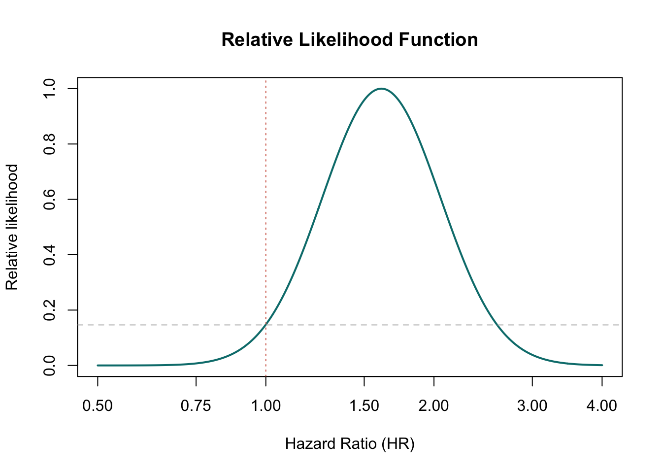
#> Number of observations (_N) was 0, now 200.
#>
#>
#>
#>
#>
#>
#>
#> Initial:      Log likelihood =  -806.4418
#> Alternative:  Log likelihood = -450.70073
#> Rescale:      Log likelihood = -429.09515
#> Rescale eq:   Log likelihood = -374.61873
#> Iteration 0:  Log likelihood = -374.61873
#> Iteration 1:  Log likelihood = -348.89609
#> Iteration 2:  Log likelihood = -343.02889
#> Iteration 3:  Log likelihood = -342.99237
#> Iteration 4:  Log likelihood = -342.99235
#>
#>                                                         Number of obs =
#> >   200
#>                                                         Wald chi2(1)  =
#> > 72.77
#> Log likelihood = -342.99235                             Prob > chi2   = 0
#> > .0000
#>
#> -------------------------------------------------------------------------
#> > -----
#>            y | Coefficient  Std. err.      z    P>|z|     [95% conf. inte
#> > rval]
#> -------------+-----------------------------------------------------------
#> > -----
#> mu           |
#>            x |   .8119551   .0951852     8.53   0.000     .6253954    .99
#> > 85147
#>        _cons |   1.868002   .0954381    19.57   0.000     1.680947    2.0
#> > 55057
#> -------------+-----------------------------------------------------------
#> > -----
#> lnsigma      |
#>        _cons |   .2960232        .05     5.92   0.000      .198025    .39
#> > 40214
#> -------------------------------------------------------------------------
#> > -----
#>
#>
#>
#>
#>
#>
#>
#>
#>
#> check: ML slope  =  0.811955  OLS slope  =  0.811955
#>
#> check: ML sigma  =  1.344501  OLS sigma (n-scaled) =  1.344501
#>
#>
#>
#> Part A validation PASSED: ml reproduces regress
#>
#>
#> Number of observations (_N) was 0, now 300.
#>
#>
#>
#>
#>
#>
#>
#> Initial:      Log likelihood = -207.94415
#> Alternative:  Log likelihood =  -205.2231
#> Rescale:      Log likelihood = -204.28183
#> Iteration 0:  Log likelihood = -204.28183
#> Iteration 1:  Log likelihood = -187.36811
#> Iteration 2:  Log likelihood = -187.34499
#> Iteration 3:  Log likelihood = -187.34499
#>
#>                                                         Number of obs =
#> >   300
#>                                                         Wald chi2(1)  =
#> > 28.32
#> Log likelihood = -187.34499                             Prob > chi2   = 0
#> > .0000
#>
#> -------------------------------------------------------------------------
#> > -----
#>            y | Coefficient  Std. err.      z    P>|z|     [95% conf. inte
#> > rval]
#> -------------+-----------------------------------------------------------
#> > -----
#>            x |   .7507449   .1410829     5.32   0.000     .4742275    1.0
#> > 27262
#>        _cons |  -.3434135    .124075    -2.77   0.006     -.586596    -.1
#> > 00231
#> -------------------------------------------------------------------------
#> > -----
#>
#>
#>
#>
#>
#>
#>
#> check: ml slope =  0.750745  logit slope =  0.750745
#>
#> check: ml ll    =  -187.344987  logit ll    =  -187.344987
#>
#>
#>
#> Part B validation PASSED: ml reproduces logit
#>
#>
#> All maximum likelihood constructions validated.
The inverse route: sweeping levels instead of parameters with cifunction
Everything above builds the curve by sweeping the parameter axis: fix a grid of candidate values, compute one (or one refit) per value, and read off a P-value. There is a second route to the same object that works from the other side: sweep the confidence level from 0 to 99.99% and compute the interval limits at each level. Plotting the limits against the levels traces exactly the same curve – the two constructions are inverse functions of each other, since the P-value function evaluated at a level’s limit returns that level’s .
A confidence interval function (also called a confidence curve, P-value function, or consonance function) displays every confidence interval around an estimate simultaneously. Ariel Linden’s cifunction Stata module implements the level-sweeping construction directly; the R equivalent is concurve. Install once from SSC:
One convention to respect: with eform, cifunction takes se() on the ratio scale (the delta-method SE, ), does its computation on the log scale, and back-transforms. Same Brown et al. example as above, with the saved output asserted against both the reported interval and the manual z-grid construction: ## Python
import numpy as np
from scipy.stats import norm
import matplotlib.pyplot as plt

point, LL, UL = 1.61, 0.997, 2.59
se = np.log(UL / LL) / (2 * 1.96)

hr = np.linspace(0.5, 4.0, 600)
z = (np.log(hr) - np.log(point)) / se

support  = np.exp(-(z**2) / 2)
deviance = z**2
pvalue   = 2 * (1 - norm.cdf(np.abs(z)))
svalue   = -np.log2(pvalue)

inside = hr[support >= 1/6.83]
assert abs(inside.min() - LL) < 0.02 and abs(inside.max() - UL) < 0.02
print("validation PASSED: 1/6.83 LI == 95% CI")
#> validation PASSED: 1/6.83 LI == 95% CI

fig, ax = plt.subplots(figsize=(7, 4.5))
ax.plot(hr, support, color="#007C7C")
ax.axvline(1, ls=":", color="#d46c5b"); ax.axhline(1/6.83, color="gray", alpha=0.4)
ax.set_xscale("log"); ax.set_xticks([0.5, 0.75, 1, 1.5, 2, 3, 4])
ax.set_xlabel("Hazard Ratio (HR)"); ax.set_ylabel("Relative likelihood")
ax.set_title("Relative Likelihood Function")
plt.show()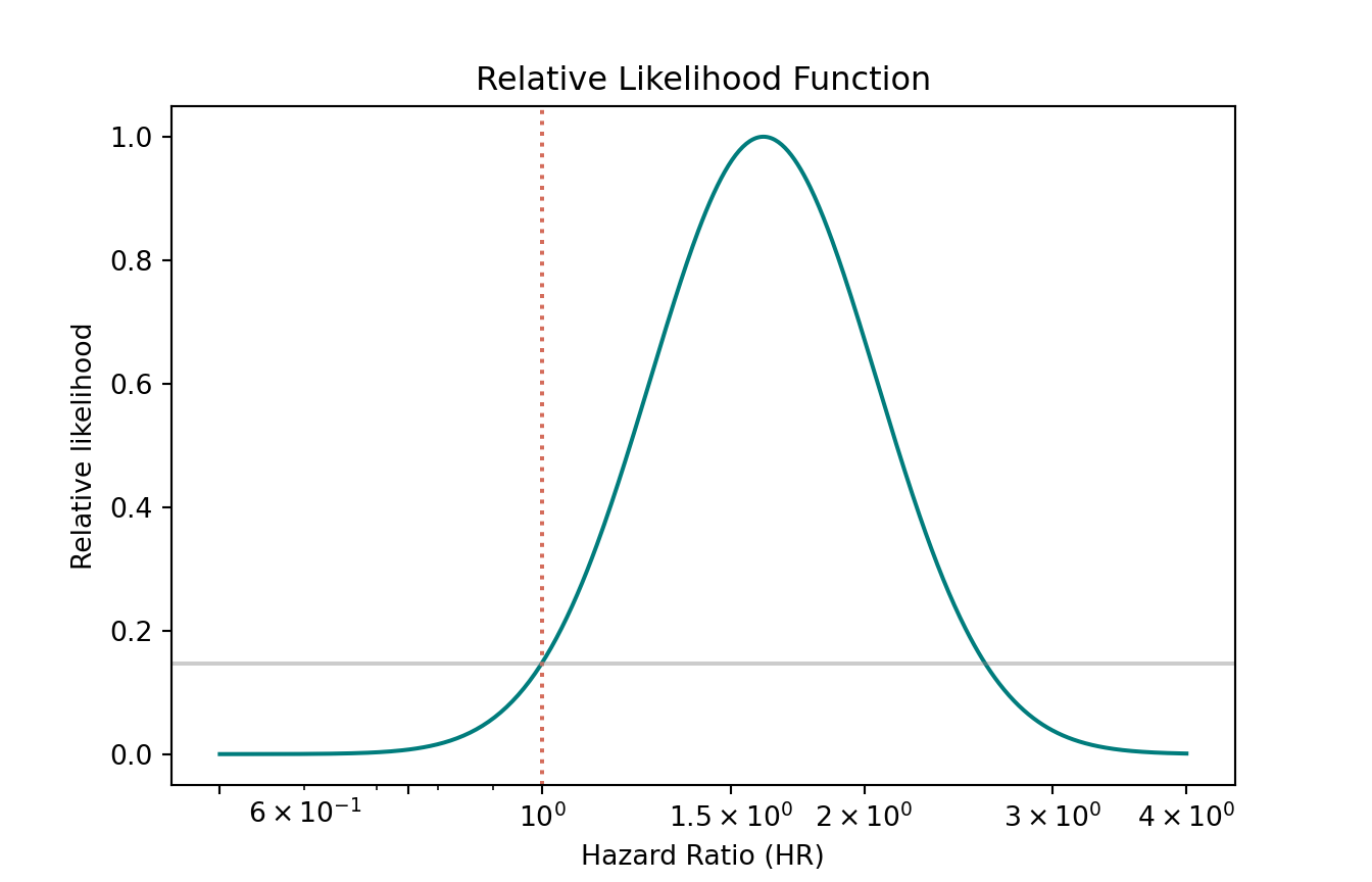
using Distributions, Plots
gr();

point, LL, UL = 1.61, 0.997, 2.59;
se = log(UL / LL) / (2 * 1.96);

hr = range(0.5, 4.0; length = 600);
z = (log.(hr) .- log(point)) ./ se;

support  = exp.(-(z .^ 2) ./ 2);
deviance = z .^ 2;
pvalue   = 2 .* (1 .- cdf.(Normal(), abs.(z)));
svalue   = .-log2.(pvalue);

inside = hr[support .>= 1/6.83];
@assert abs(minimum(inside) - LL) < 0.02 && abs(maximum(inside) - UL) < 0.02
println("validation PASSED: 1/6.83 LI == 95% CI")
#> validation PASSED: 1/6.83 LI == 95% CI

p = plot(hr, support; xscale = :log10, legend = false,
         xlabel = "Hazard Ratio (HR)", ylabel = "Relative likelihood",
         title = "Relative Likelihood Function");
hline!(p, [1/6.83]; color = :gray, alpha = 0.4);
vline!(p, [1.0]; linestyle = :dot, color = :red);
p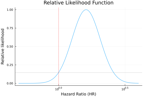
normcdf needs the Statistics Toolbox; the erfc form below is base MATLAB and gives the identical two-sided tail, so this tab runs either way.
point = 1.61; LL = 0.997; UL = 2.59;
se = log(UL / LL) / (2 * 1.96);

hr = linspace(0.5, 4.0, 600)';
z  = (log(hr) - log(point)) / se;

support  = exp(-(z.^2) / 2);
deviance = z.^2;
% two-sided p; erfc form avoids the Statistics Toolbox dependency
pvalue   = erfc(abs(z) / sqrt(2));
svalue   = -log2(pvalue);

inside = hr(support >= 1/6.83);
assert(abs(min(inside) - LL) < 0.02 && abs(max(inside) - UL) < 0.02)
disp('validation PASSED: 1/6.83 LI == 95% CI')

figure;
semilogx(hr, support, 'LineWidth', 2, 'Color', [0 0.486 0.486]);
xticks([0.5 0.75 1 1.5 2 3 4]);
xline(1,      ':', 'Color', [0.831 0.424 0.357]);
yline(1/6.83, '--', 'Color', [0.5 0.5 0.5]);
xlabel('Hazard Ratio (HR)'); ylabel('Relative likelihood');
title('Relative Likelihood Function');
Neither Snowflake nor DuckDB ships erf(), so uses the Abramowitz–Stegun 26.2.17 polynomial ( per tail). SQL does not plot; it returns a table, and something else draws it – Power BI, or in this case R.
WITH params AS (
  SELECT 1.61::DOUBLE AS point,
         ln(2.59 / 0.997) / (2 * 1.96) AS se
),
grid AS (
  SELECT 0.5 + (i - 1) * (4.0 - 0.5) / 599 AS hr
  FROM generate_series(1, 600) AS t(i)
),
lik AS (
  SELECT g.hr,
         (ln(g.hr) - ln(p.point)) / p.se                     AS z,
         exp(-power((ln(g.hr) - ln(p.point)) / p.se, 2) / 2) AS support,
         power((ln(g.hr) - ln(p.point)) / p.se, 2)           AS deviance
  FROM grid g CROSS JOIN params p
),
pv AS (
  SELECT hr, z, support, deviance,
         2 * ( exp(-z*z/2) / sqrt(2*pi()) *
               ( 0.319381530 * (1/(1 + 0.2316419*abs(z)))
               - 0.356563782 * power(1/(1 + 0.2316419*abs(z)), 2)
               + 1.781477937 * power(1/(1 + 0.2316419*abs(z)), 3)
               - 1.821255978 * power(1/(1 + 0.2316419*abs(z)), 4)
               + 1.330274429 * power(1/(1 + 0.2316419*abs(z)), 5) ) ) AS pvalue
  FROM lik
)
SELECT hr, support, deviance, pvalue, -ln(pvalue)/ln(2) AS svalue
FROM pv ORDER BY hr LIMIT 5;| hr | support | deviance | pvalue | svalue |
|---|---|---|---|---|
| 0.500 | 0 | 23.1 | 0 | 19.3 |
| 0.506 | 0 | 22.6 | 0 | 18.9 |
| 0.512 | 0 | 22.2 | 0 | 18.6 |
| 0.518 | 0 | 21.7 | 0 | 18.3 |
| 0.523 | 0 | 21.3 | 0 | 17.9 |
All four coordinate views come out of that one query. The interval it returns is against the reported , and the Abramowitz–Stegun polynomial tracks R’s pnorm to :
cur <- DBI::dbGetQuery(con, "
  WITH params AS (SELECT 1.61::DOUBLE AS point, ln(2.59/0.997)/(2*1.96) AS se),
  grid AS (SELECT 0.5 + (i-1)*(4.0-0.5)/599 AS hr FROM generate_series(1,600) AS t(i)),
  lik AS (SELECT g.hr, (ln(g.hr)-ln(p.point))/p.se AS z,
                 exp(-power((ln(g.hr)-ln(p.point))/p.se,2)/2) AS support,
                 power((ln(g.hr)-ln(p.point))/p.se,2) AS deviance
          FROM grid g CROSS JOIN params p),
  pv AS (SELECT hr, z, support, deviance,
           2 * ( exp(-z*z/2)/sqrt(2*pi()) *
             ( 0.319381530*(1/(1+0.2316419*abs(z)))
             - 0.356563782*power(1/(1+0.2316419*abs(z)),2)
             + 1.781477937*power(1/(1+0.2316419*abs(z)),3)
             - 1.821255978*power(1/(1+0.2316419*abs(z)),4)
             + 1.330274429*power(1/(1+0.2316419*abs(z)),5) ) ) AS pvalue
         FROM lik)
  SELECT hr, support, deviance, pvalue, -ln(pvalue)/ln(2) AS svalue
  FROM pv ORDER BY hr;")

inside <- cur$hr[cur$support >= 1/6.83]
exact  <- 2 * (1 - pnorm(abs((log(cur$hr) - log(1.61)) /
                             (log(2.59/0.997)/(2*1.96)))))
stopifnot(abs(min(inside) - 0.997) < 0.02, abs(max(inside) - 2.59) < 0.02,
          max(abs(cur$pvalue - exact)) < 1e-6)
cat(sprintf("1/6.83 interval: [%.4f, %.4f]\n", min(inside), max(inside)))
#> 1/6.83 interval: [1.0025, 2.5918]
cat(sprintf("max |Abramowitz-Stegun - pnorm| = %.2e\n",
            max(abs(cur$pvalue - exact))))
#> max |Abramowitz-Stegun - pnorm| = 1.49e-07
cat(sprintf("S-value at HR = 1: %.2f bits\n",
            cur$svalue[which.min(abs(cur$hr - 1))]))
#> S-value at HR = 1: 4.27 bits

op <- par(mfrow = c(2, 2), mar = c(4, 4, 2.5, 1))
panel <- function(y, ylab, main, href = NA) {
  plot(cur$hr, y, type = "l", log = "x", col = "#007C7C", lwd = 2,
       xaxt = "n", xlab = "Hazard Ratio", ylab = ylab, main = main)
  axis(1, at = c(0.5, 1, 2, 4))
  abline(v = 1, lty = 3, col = "#d46c5b")
  if (!is.na(href)) abline(h = href, col = "gray", lty = 2)
}
panel(cur$support,  "Relative likelihood", "Support",   1/6.83)
panel(cur$deviance, "Deviance",            "Deviance",  3.84)
panel(cur$pvalue,   "P-value",             "P-value (compatibility)", 0.05)
panel(cur$svalue,   "Bits of information", "S-value",   4.32)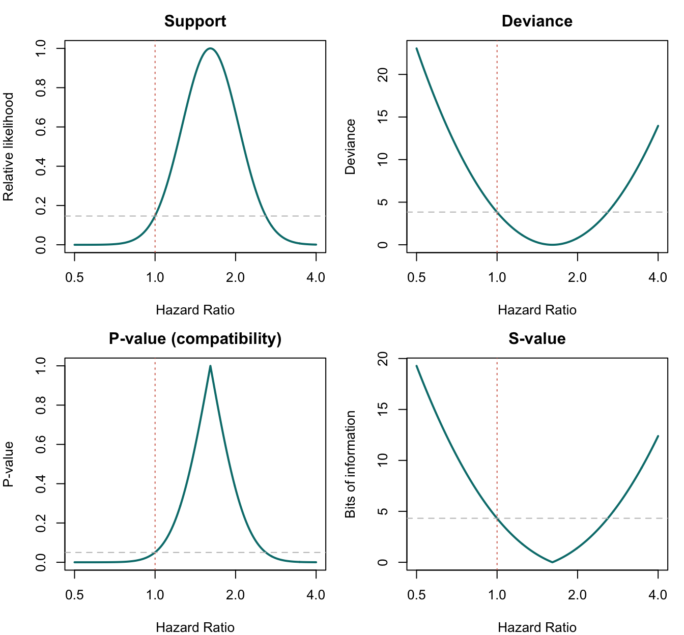
par(op)The dotted vertical line marks HR . Reading the bottom-right panel: the S-value there is 4.27 bits – about as much evidence against the null as five straight heads, which is not much.
Profile likelihood for a regression coefficient
The offset trick: to fix the coefficient of at , move into an offset and refit the model without . The refit re-maximizes the intercept and the other covariates at every grid point – that is what makes it a profile likelihood rather than a slice through the likelihood at the MLEs.
set.seed(1031)
n <- 300
x <- rnorm(n)
w <- rnorm(n)
y <- as.numeric(runif(n) < plogis(-0.3 + 0.8*x + 0.4*w))

full  <- glm(y ~ x + w, family = binomial())
bhat  <- coef(full)[["x"]]
sehat <- sqrt(diag(vcov(full)))[["x"]]

# offset trick: fix the coefficient of x at b and refit without x, so the
# intercept and w are re-maximized at every grid point
grid <- seq(bhat - 4*sehat, bhat + 4*sehat, length.out = 121)
ll <- vapply(grid, function(b)
  as.numeric(logLik(glm(y ~ w, family = binomial(), offset = b*x))),
  numeric(1))

support  <- exp(ll - max(ll))
deviance <- -2*(ll - max(ll))

stopifnot(abs(grid[which.max(support)] - bhat) < diff(grid)[1])
cat("validation PASSED: profile peak == full-model MLE\n")
#> validation PASSED: profile peak == full-model MLE

si <- range(grid[support >= 1/6.83])
cat(sprintf("1/6.83 support interval: [%.4f, %.4f]   Wald 95%% CI: [%.4f, %.4f]\n",
            si[1], si[2], bhat - 1.96*sehat, bhat + 1.96*sehat))
#> 1/6.83 support interval: [0.5593, 1.1148]   Wald 95% CI: [0.5459, 1.1090]

plot(grid, support, type = "l", col = "#007C7C", lwd = 2,
     xlab = "Coefficient of x (log-odds scale)",
     ylab = "Relative likelihood",
     main = "Profile Likelihood Function")
abline(v = bhat, lty = 2, col = "gray40")
abline(h = 1/6.83, col = "gray", lty = 2)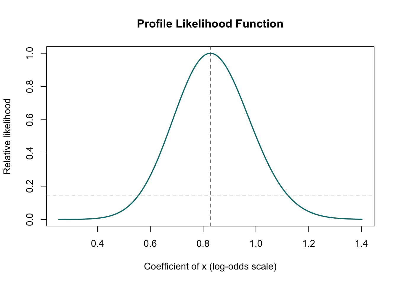
#> Number of observations (_N) was 0, now 300.
#>
#>
#>
#>
#>
#>
#>
#>
#>
#>
#>
#>
#>
#> (file /var/folders/p4/rr9th0593k1_k0bf90vnc57w0000gn/T//S_81015.000001
#>     not found)
#>
#>
#>
#>
#>
#>
#>
#>
#>
#> profile peak =  0.748198   full-model MLE =  0.748198
#>
#>
#>
#> 1/6.83 support interval: [0.4730, 1.0430]   Wald 95% CI: [0.4593, 1.0371]
#>
#>
#>
#> Part B validation PASSED: profile peak and support interval check out
#>
#>
#>
#>
#> file profile_likelihood_logit.svg saved as SVG format
#>
#>
#> All likelihood-function constructions validated.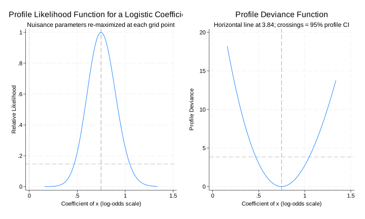
import numpy as np
import statsmodels.api as sm
import matplotlib.pyplot as plt

rng = np.random.default_rng(1031)
n = 300
x = rng.normal(0, 1, n)
w = rng.normal(0, 1, n)
y = (rng.uniform(size=n) < 1/(1 + np.exp(-(-0.3 + 0.8*x + 0.4*w)))).astype(float)

X_full = sm.add_constant(np.column_stack([x, w]))
full = sm.GLM(y, X_full, family=sm.families.Binomial()).fit()
bhat, sehat = full.params[1], full.bse[1]
X_nuis = sm.add_constant(w)

grid = np.linspace(bhat - 4*sehat, bhat + 4*sehat, 121)
ll = np.array([
    sm.GLM(y, X_nuis, family=sm.families.Binomial(), offset=b*x).fit().llf
    for b in grid
])
support = np.exp(ll - ll.max())

assert abs(grid[np.argmax(support)] - bhat) < grid[1] - grid[0]
print("validation PASSED: profile peak == full-model MLE")
#> validation PASSED: profile peak == full-model MLE

fig, ax = plt.subplots(figsize=(7, 4.5))
ax.plot(grid, support, color="#007C7C")
ax.axvline(bhat, ls="--", color="gray")
ax.axhline(1/6.83, color="gray", alpha=0.4)
ax.set_xlabel("Coefficient of x (log-odds)")
ax.set_ylabel("Relative likelihood")
ax.set_title("Profile Likelihood Function")
plt.show()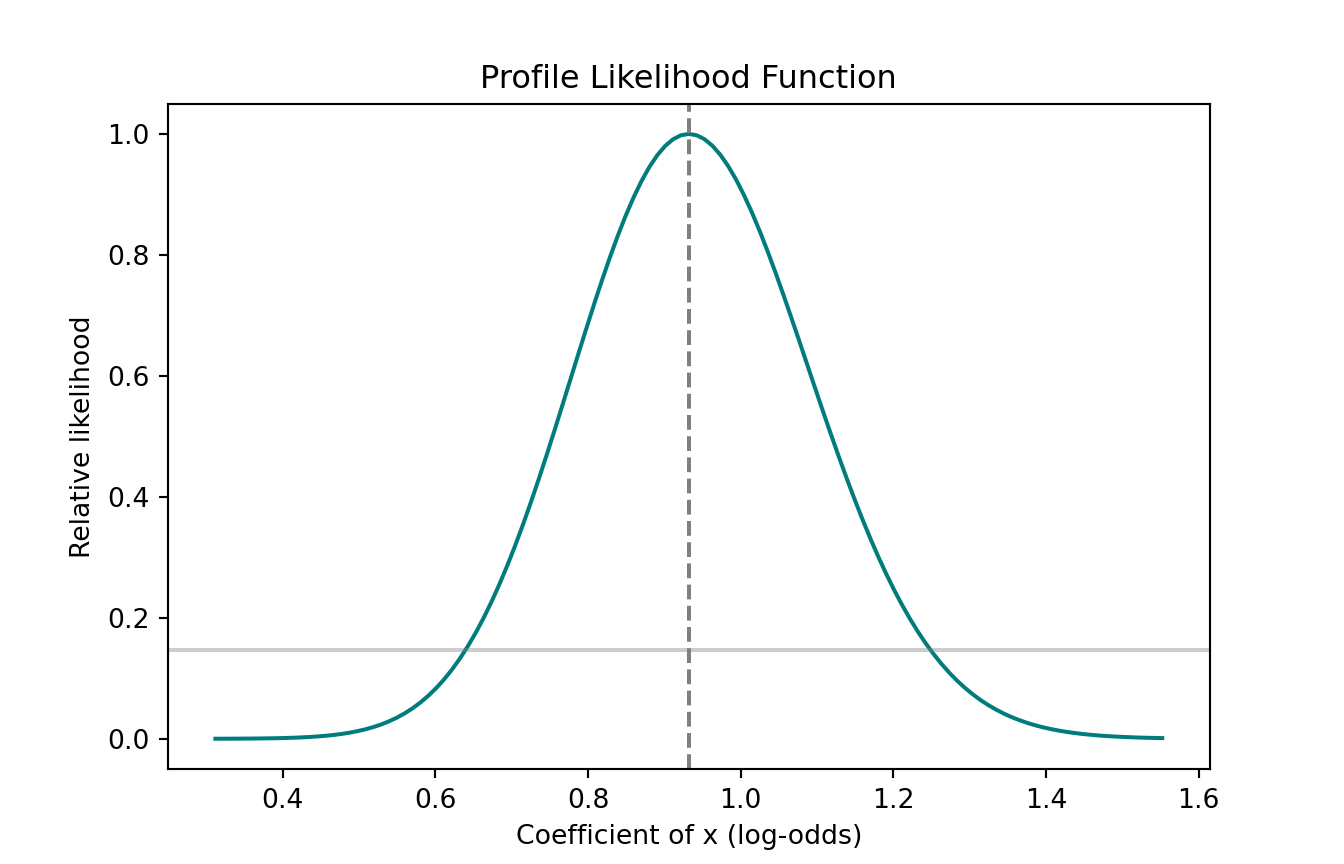
using Distributions, GLM, DataFrames, Random, Plots

rng = MersenneTwister(1031);
n = 300;
x = randn(rng, n);
w = randn(rng, n);
y = Float64.(rand(rng, n) .< 1 ./ (1 .+ exp.(-(-0.3 .+ 0.8 .* x .+ 0.4 .* w))));
df = DataFrame(y = y, x = x, w = w)
#> 300×3 DataFrame
#>  Row │ y        x            w
#>      │ Float64  Float64      Float64
#> ─────┼──────────────────────────────────
#>    1 │     0.0   1.53733      0.212606
#>    2 │     1.0   0.67567      2.18329
#>    3 │     0.0   0.529915    -0.411984
#>    4 │     0.0  -0.469345     0.243801
#>    5 │     0.0  -0.344731     0.181979
#>    6 │     1.0   0.00596521   0.102878
#>    7 │     0.0  -1.52318     -0.446261
#>    8 │     1.0   0.390072    -1.61528
#>   ⋮  │    ⋮          ⋮           ⋮
#>  294 │     1.0  -1.21183      0.133128
#>  295 │     1.0   0.35636     -0.373798
#>  296 │     1.0   0.125155     0.561362
#>  297 │     0.0  -1.63194     -0.0784788
#>  298 │     0.0  -0.464039    -0.214666
#>  299 │     1.0   1.21094     -0.392618
#>  300 │     1.0  -1.2263      -0.228791
#>                         285 rows omitted

full = glm(@formula(y ~ x + w), df, Binomial(), LogitLink())
#> StatsModels.TableRegressionModel{GeneralizedLinearModel{GLM.GlmResp{Vector{Float64}, Binomial{Float64}, LogitLink}, GLM.DensePredChol{Float64, CholeskyPivoted{Float64, Matrix{Float64}, Vector{Int64}}}}, Matrix{Float64}}
#>
#> y ~ 1 + x + w
#>
#> Coefficients:
#> ─────────────────────────────────────────────────────────────────────────
#>                  Coef.  Std. Error      z  Pr(>|z|)  Lower 95%  Upper 95%
#> ─────────────────────────────────────────────────────────────────────────
#> (Intercept)  -0.378416    0.133353  -2.84    0.0045  -0.639782  -0.117049
#> x             1.07021     0.160245   6.68    <1e-10   0.756132   1.38428
#> w             0.475207    0.130953   3.63    0.0003   0.218545   0.73187
#> ─────────────────────────────────────────────────────────────────────────
bhat, sehat = coef(full)[2], stderror(full)[2];

grid = range(bhat - 4*sehat, bhat + 4*sehat; length = 121);
ll = [loglikelihood(glm(@formula(y ~ w), df, Binomial(), LogitLink();
                        offset = b .* x)) for b in grid];
support = exp.(ll .- maximum(ll));

@assert abs(grid[argmax(support)] - bhat) < grid[2] - grid[1]
println("validation PASSED: profile peak == full-model MLE")
#> validation PASSED: profile peak == full-model MLE

p = plot(grid, support; legend = false,
         xlabel = "Coefficient of x (log-odds)",
         ylabel = "Relative likelihood",
         title = "Profile Likelihood Function");
vline!(p, [bhat]; linestyle = :dash, color = :gray);
hline!(p, [1/6.83]; color = :gray, alpha = 0.4);
p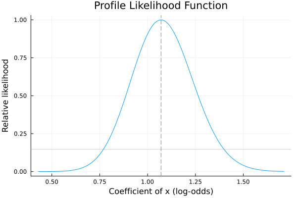
glmfit takes an 'Offset' name–value pair, so the offset trick carries over directly: fix the coefficient of at , push into the offset, and refit on alone so the intercept and are re-maximized at every point.
rng(1031, 'twister');
n = 300;
x = randn(n, 1);
w = randn(n, 1);
y = double(rand(n,1) < 1 ./ (1 + exp(-(-0.3 + 0.8*x + 0.4*w))));

% full fit: MLE and Wald SE define the grid
[b_full, ~, stats] = glmfit([x w], y, 'binomial', 'link', 'logit');
bhat  = b_full(2);
sehat = stats.se(2);

grid = linspace(bhat - 4*sehat, bhat + 4*sehat, 121)';
ll   = zeros(size(grid));
for k = 1:numel(grid)
    % offset fixes b*x; only the intercept and w are re-estimated
    [~, dev] = glmfit(w, y, 'binomial', 'link', 'logit', ...
                      'Offset', grid(k)*x);
    ll(k) = -dev / 2;   % glmfit returns deviance = -2*loglik (up to a constant)
end

support  = exp(ll - max(ll));
deviance = -2*(ll - max(ll));

[~, imax] = max(support);
assert(abs(grid(imax) - bhat) < grid(2) - grid(1))
disp('validation PASSED: profile peak == full-model MLE')

si = [min(grid(support >= 1/6.83)), max(grid(support >= 1/6.83))];
fprintf('1/6.83 support interval: [%.4f, %.4f]   Wald 95%% CI: [%.4f, %.4f]\n', ...
        si(1), si(2), bhat - 1.96*sehat, bhat + 1.96*sehat);

figure;
plot(grid, support, 'LineWidth', 2, 'Color', [0 0.486 0.486]);
xline(bhat,   '--', 'Color', [0.4 0.4 0.4]);
yline(1/6.83, '--', 'Color', [0.5 0.5 0.5]);
xlabel('Coefficient of x (log-odds scale)');
ylabel('Relative likelihood');
title('Profile Likelihood Function');
For the binomial family glmfit’s deviance is up to an additive constant that does not depend on the parameters, so it cancels in ll - max(ll) – which is all the relative likelihood needs.
SQL cannot iteratively refit a GLM (no IRLS), so a logistic profile is out of scope. But for the normal linear model the conditional MLEs of the intercept and given a fixed slope are closed-form, so profiling collapses to one AVG per candidate slope – a GROUP BY, not a refit loop. The profile-grid MLE matches REGR_SLOPE exactly here – the peak and the closed form agree to the last printed digit, since both are computed from the same rows. (Dialect landmine: Snowflake rejects correlated scalar subqueries here; the CROSS JOIN + GROUP BY below is the working idiom.)
-- One AVG per candidate slope: profiling collapses to a GROUP BY because the
-- conditional MLEs of the intercept and sigma^2 given a fixed slope are
-- closed-form. No refit loop, no IRLS.
WITH closed AS (
  SELECT regr_slope(y, x) AS b1, count(*) AS n FROM mytable
),
m AS (
  SELECT avg(x) AS xbar, avg(y) AS ybar FROM mytable
),
grid AS (
  SELECT c.b1 - 0.3 + (g.i - 1) * 0.6 / 400 AS b_cand
  FROM generate_series(1, 401) AS g(i) CROSS JOIN closed c
),
prof AS (
  SELECT g.b_cand,
         -(c.n / 2.0) *
         ln(avg(power(d.y - (m.ybar - g.b_cand * m.xbar)
                          - g.b_cand * d.x, 2))) AS prof_loglik
  FROM grid g
  CROSS JOIN mytable d
  CROSS JOIN m
  CROSS JOIN closed c
  GROUP BY g.b_cand, c.n
)
SELECT b_cand,
       exp(prof_loglik - max(prof_loglik) OVER ()) AS support
FROM prof ORDER BY b_cand LIMIT 5;| b_cand | support |
|---|---|
| 0.295 | 0.012 |
| 0.297 | 0.013 |
| 0.298 | 0.013 |
| 0.300 | 0.014 |
| 0.301 | 0.014 |
That returns all 401 grid points (truncated to five above). SQL has no plotting layer, so hand the result set to whatever draws your charts – here, R:
prof <- DBI::dbGetQuery(con, "
  WITH closed AS (SELECT regr_slope(y,x) AS b1, count(*) AS n FROM mytable),
  m AS (SELECT avg(x) AS xbar, avg(y) AS ybar FROM mytable),
  grid AS (SELECT c.b1 - 0.3 + (g.i-1) * 0.6/400 AS b_cand
           FROM generate_series(1,401) AS g(i) CROSS JOIN closed c),
  prof AS (
    SELECT g.b_cand,
           -(c.n/2.0) * ln(avg(power(d.y - (m.ybar - g.b_cand*m.xbar)
                                         - g.b_cand*d.x, 2))) AS prof_loglik
    FROM grid g CROSS JOIN mytable d CROSS JOIN m CROSS JOIN closed c
    GROUP BY g.b_cand, c.n)
  SELECT b_cand, exp(prof_loglik - max(prof_loglik) OVER ()) AS support
  FROM prof ORDER BY b_cand;")

b1_sql <- sql$b1
peak   <- prof$b_cand[which.max(prof$support)]
si     <- range(prof$b_cand[prof$support >= 1/6.83])
ci     <- confint(ols, "x", level = 0.95)

# the two self-checks from the top of the post
stopifnot(abs(peak - b1_sql) < diff(prof$b_cand)[1])
cat(sprintf("profile peak = %.10f   REGR_SLOPE = %.10f\n", peak, b1_sql))
#> profile peak = 0.5953684349   REGR_SLOPE = 0.5953684349
cat(sprintf("1/6.83 support interval: [%.4f, %.4f]\n", si[1], si[2]))
#> 1/6.83 support interval: [0.3989, 0.7919]
cat(sprintf("lm 95%% CI:               [%.4f, %.4f]\n", ci[1], ci[2]))
#> lm 95% CI:               [0.3974, 0.7933]

plot(prof$b_cand, prof$support, type = "l", col = "#007C7C", lwd = 2,
     xlab = "Candidate slope", ylab = "Relative likelihood",
     main = "Profile Likelihood Computed Entirely in SQL")
abline(v = b1_sql, lty = 2, col = "gray40")
abline(h = 1/6.83, col = "gray", lty = 2)
segments(si[1], 1/6.83, si[2], 1/6.83, col = "#d46c5b", lwd = 3)
text(b1_sql, 0.55, "REGR_SLOPE", cex = 0.75, col = "gray30", pos = 4)
text(mean(si), 1/6.83 - 0.055, "1/6.83 support interval",
     cex = 0.75, col = "#d46c5b")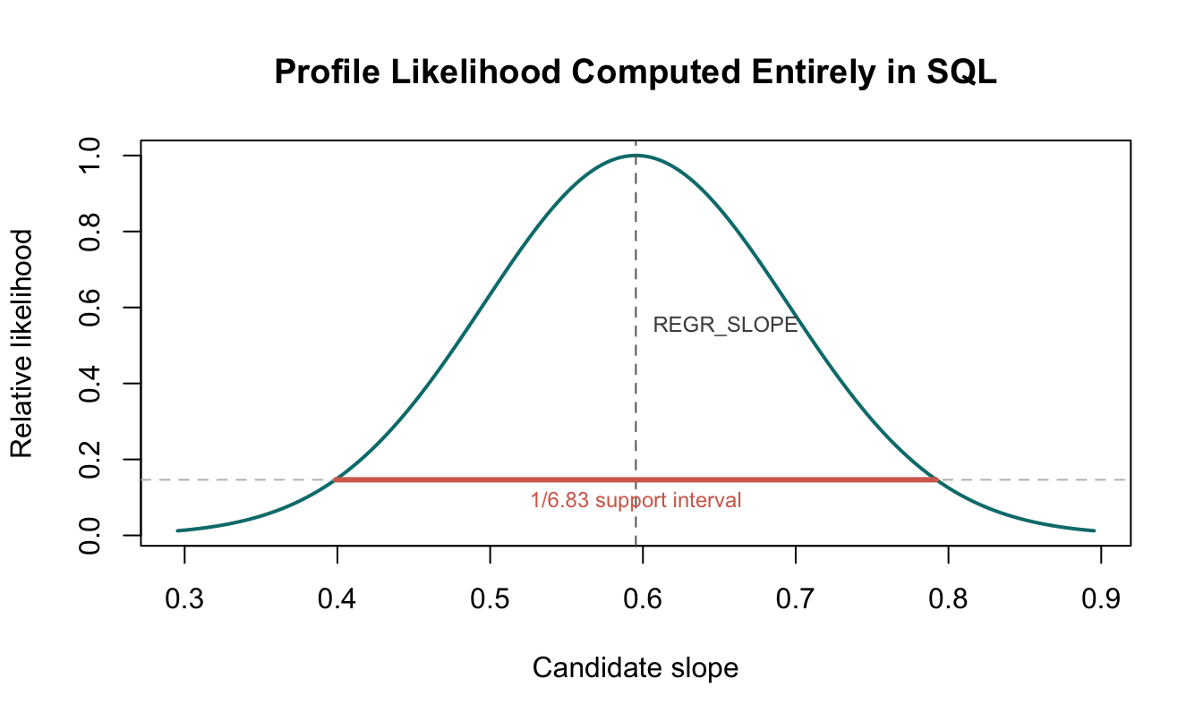
The support interval drawn in orange and the Wald interval from lm agree to about three decimals, which is the same identity the R, Python, and Julia sections check – here with every number produced by a GROUP BY.
Existing R tools as alternatives
Everything above builds the likelihood by hand. In R you usually do not have to: several packages will do the maximizing and profiling for you, and their output reshapes into the same five-column object concurve plots. The one helper below is all the glue needed. See the concurve vignettes on likelihood tools and profile likelihoods for the longer treatment.
library(concurve)

# Reshape any (parameter grid, log-likelihood) pair into concurve's format.
as_concurve_lik <- function(values, loglik) {
  loglik_rel <- loglik - max(loglik)
  support    <- exp(loglik_rel)
  df <- data.frame(
    values        = values,
    likelihood    = support,
    loglikelihood = loglik_rel,
    support       = support,
    deviancestat  = -loglik_rel
  )
  class(df) <- c("data.frame", "concurve")
  df
}

set.seed(123)
x <- rnorm(50, mean = 9.3, sd = 3.2)
c(mean = mean(x), sd = sd(x))
#> mean   sd
#> 9.41 2.96Base R, no dependencies. optim finds the MLE and the Hessian gives Wald standard errors. To profile , substitute the conditional MLE of at each grid point rather than holding fixed.
nll_normal <- function(theta, x) {
  mu <- theta[1]; sigma <- theta[2]
  -sum(dnorm(x, mean = mu, sd = sigma, log = TRUE))
}

fit <- optim(c(mu = 8, sigma = 3), nll_normal, x = x,
             method = "BFGS", hessian = TRUE)
fit$par
#>    mu sigma
#>  9.41  2.93
sqrt(diag(solve(fit$hessian)))
#>    mu sigma
#> 0.415 0.293

n <- length(x)
mu_grid <- seq(fit$par["mu"] - 3, fit$par["mu"] + 3, length.out = 4000)
loglik_mu <- vapply(mu_grid, function(m) {
  sigma2_hat <- mean((x - m)^2)          # conditional MLE of sigma^2 given mu
  -(n / 2) * (log(2 * pi) + log(sigma2_hat) + 1)
}, numeric(1))

lik_optim <- as_concurve_lik(mu_grid, loglik_mu)
stopifnot(abs(mu_grid[which.max(loglik_mu)] - fit$par[["mu"]]) < 1e-2)

ggcurve(lik_optim, type = "l1", nullvalue = round(fit$par[["mu"]], 2),
        xaxis = expression(mu),
        title = "Likelihood for the Mean (via optim profiling)")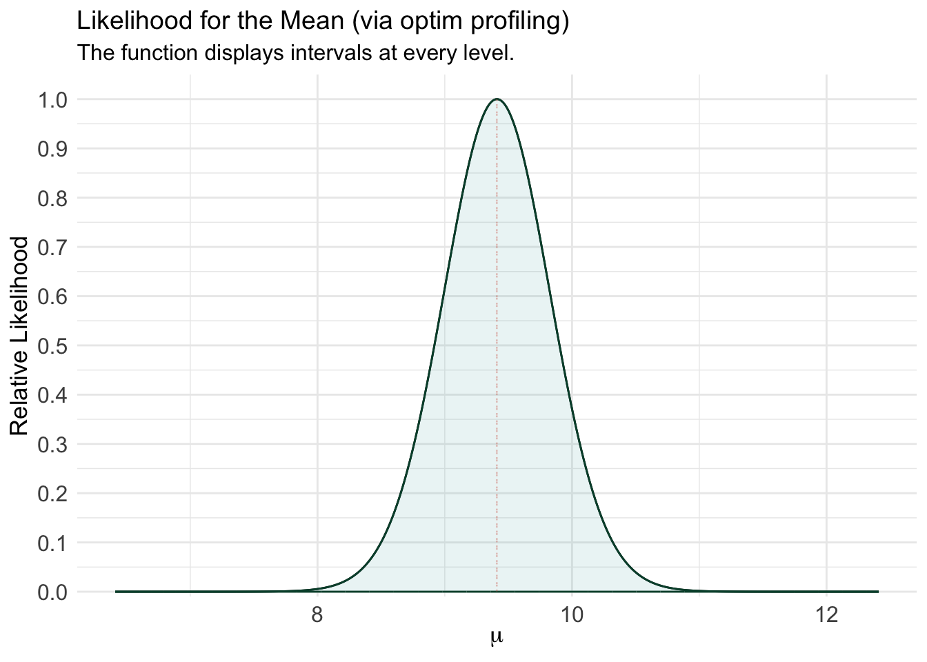
maxLik maximizes the log-likelihood directly, with no sign flipping, and prints a summary with standard errors.
library(maxLik)

loglik_normal <- function(theta, x) {
  sum(dnorm(x, mean = theta[1], sd = sqrt(theta[2]), log = TRUE))
}
theta_mle <- maxLik(loglik_normal, start = c(mu = 8, sig2 = 9), x = x)
summary(theta_mle)
#> --------------------------------------------
#> Maximum Likelihood estimation
#> Newton-Raphson maximisation, 7 iterations
#> Return code 8: successive function values within relative tolerance limit (reltol)
#> Log-Likelihood: -125
#> 2  free parameters
#> Estimates:
#>      Estimate Std. error t value Pr(> t)
#> mu      9.410      0.415   22.66 < 2e-16 ***
#> sig2    8.602      1.712    5.02 5.1e-07 ***
#> ---
#> Signif. codes:  0 ‘***’ 0.001 ‘**’ 0.01 ‘*’ 0.05 ‘.’ 0.1 ‘ ’ 1
#> --------------------------------------------

loglik_mu2 <- vapply(mu_grid, function(m) {
  loglik_normal(c(m, mean((x - m)^2)), x = x)
}, numeric(1))

stopifnot(abs(coef(theta_mle)[[1]] - fit$par[["mu"]]) < 1e-3)

ggcurve(as_concurve_lik(mu_grid, loglik_mu2), type = "l1",
        nullvalue = round(coef(theta_mle)[[1]], 2),
        xaxis = expression(mu),
        title = "Likelihood for the Mean (via maxLik)")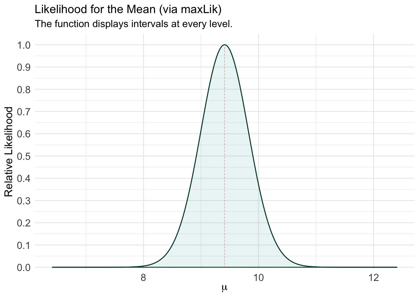
bbmle::mle2 is the only route here that profiles for you. profile() returns the signed square-root deviance , so the relative log-likelihood is .
library(bbmle)

nll <- function(mu, sigma) -sum(dnorm(x, mean = mu, sd = sigma, log = TRUE))
m <- mle2(nll, start = list(mu = 8, sigma = 3), data = list(x = x))

pr    <- profile(m)
pr_mu <- as.data.frame(pr)
pr_mu <- pr_mu[pr_mu$param == "mu", ]

mu_vals <- pr_mu[["par.vals.mu"]]
if (is.null(mu_vals)) mu_vals <- pr_mu[["mu"]]

lik_bbmle <- as_concurve_lik(mu_vals, -0.5 * pr_mu$z^2)
stopifnot(abs(coef(m)[["mu"]] - fit$par[["mu"]]) < 1e-3)

ggcurve(lik_bbmle, type = "l1", nullvalue = round(coef(m)[["mu"]], 2),
        xaxis = expression(mu),
        title = "Profile Likelihood for the Mean (via bbmle)")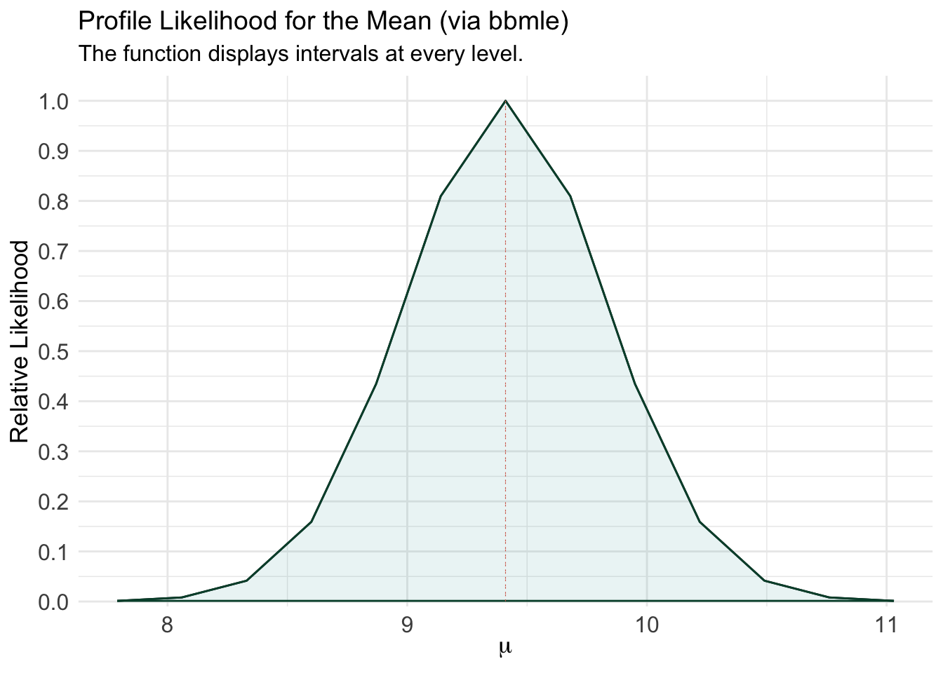
For a binary outcome carrying many nuisance parameters, cond gives exact conditional likelihood inference: it conditions the nuisance parameters out instead of profiling them.
library(cond)
data(babies)

mod_babies <- glm(cbind(r1, r2) ~ day + lull - 1,
                  family = binomial, data = babies)
cond_fit <- cond(mod_babies, offset = lullyes)
summary(cond_fit)
#>
#>  Formula:  cbind(r1, r2) ~ day + lull - 1
#>  Family:  binomial
#>  Offset:  lullyes
#>
#>           Estimate   Std. Error
#> uncond.        1.43        0.734
#> cond.          1.27        0.689
#>
#> Confidence intervals
#> --------------------
#>  level = 95 %
#>                                            lower two-sided upper
#> Wald pivot                              -0.00651            2.87
#> Wald pivot (cond. MLE)                  -0.08020            2.62
#> Likelihood root                          0.12300            3.09
#> Modified likelihood root                 0.01070            2.76
#> Modified likelihood root (cont. corr.)  -0.15200            3.10
#>
#> Diagnostics:
#> -----------
#>   INF    NP
#> 0.076 0.289
#>
#>  Approximation based on 20 points
plot(cond_fit, which = 2)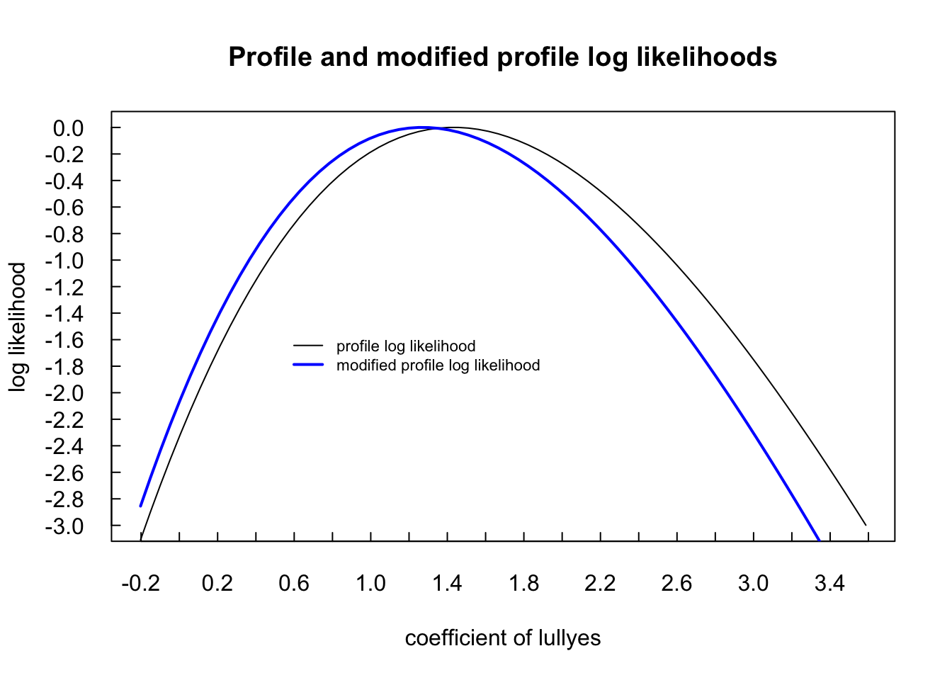
The pitfall: slicing is not profiling
Fixing a nuisance parameter instead of re-maximizing it is the most common way to get this wrong. Holding here yields a likelihood far too narrow, because the real is about 3.2 — the interval it implies is roughly a third of the honest width:
loglik_slice <- vapply(mu_grid, function(m) -0.5 * sum((x - m)^2), numeric(1))
lik_slice    <- as_concurve_lik(mu_grid, loglik_slice)

w <- function(o) {
  s <- curve_support(o, 6.83)
  s$upper.limit - s$lower.limit
}
c(slice_width = w(lik_slice), profile_width = w(lik_optim))
#>   slice_width profile_width
#>         0.554         1.658
stopifnot(w(lik_slice) < w(lik_optim))

ggcurve(lik_slice, type = "l1", nullvalue = round(fit$par[["mu"]], 2),
        xaxis = expression(mu),
        title = "WRONG: mean likelihood with sigma^2 fixed at 1",
        subtitle = "Too narrow -- the real sigma is about 3.2, not 1")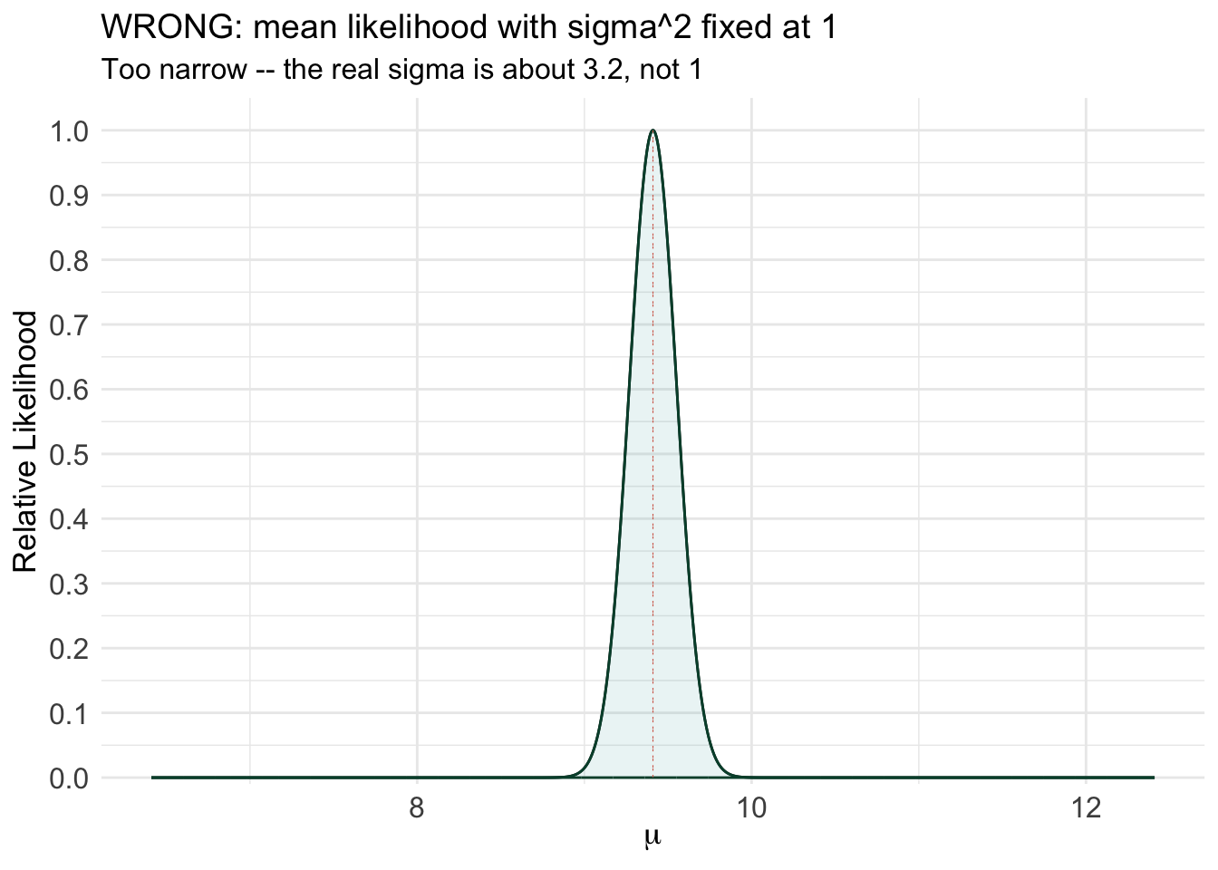
Profile likelihood from ProfileLikelihood
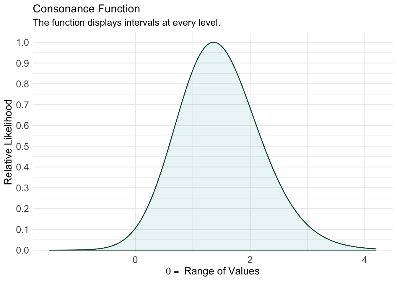
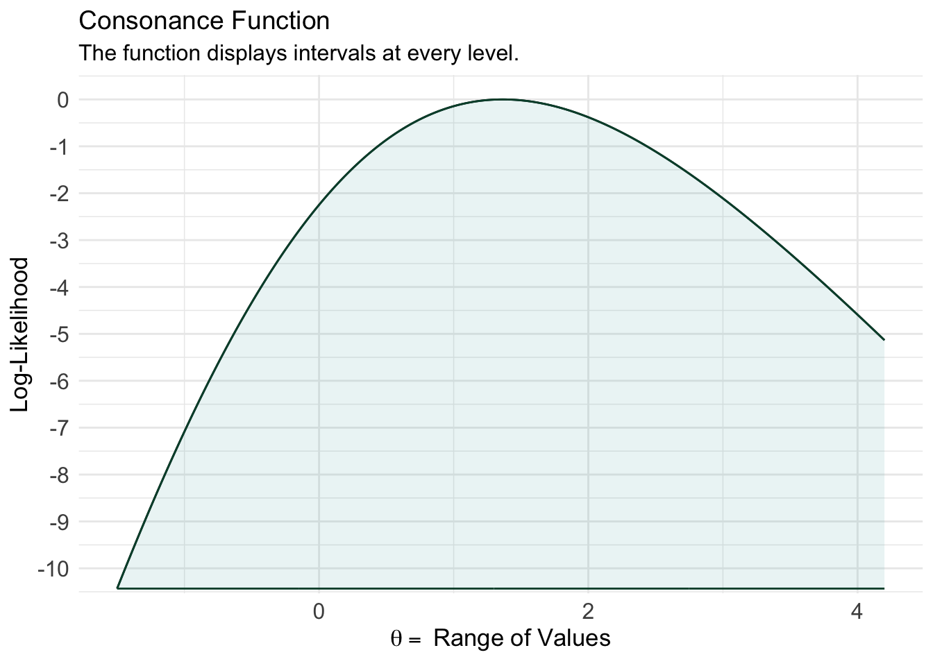
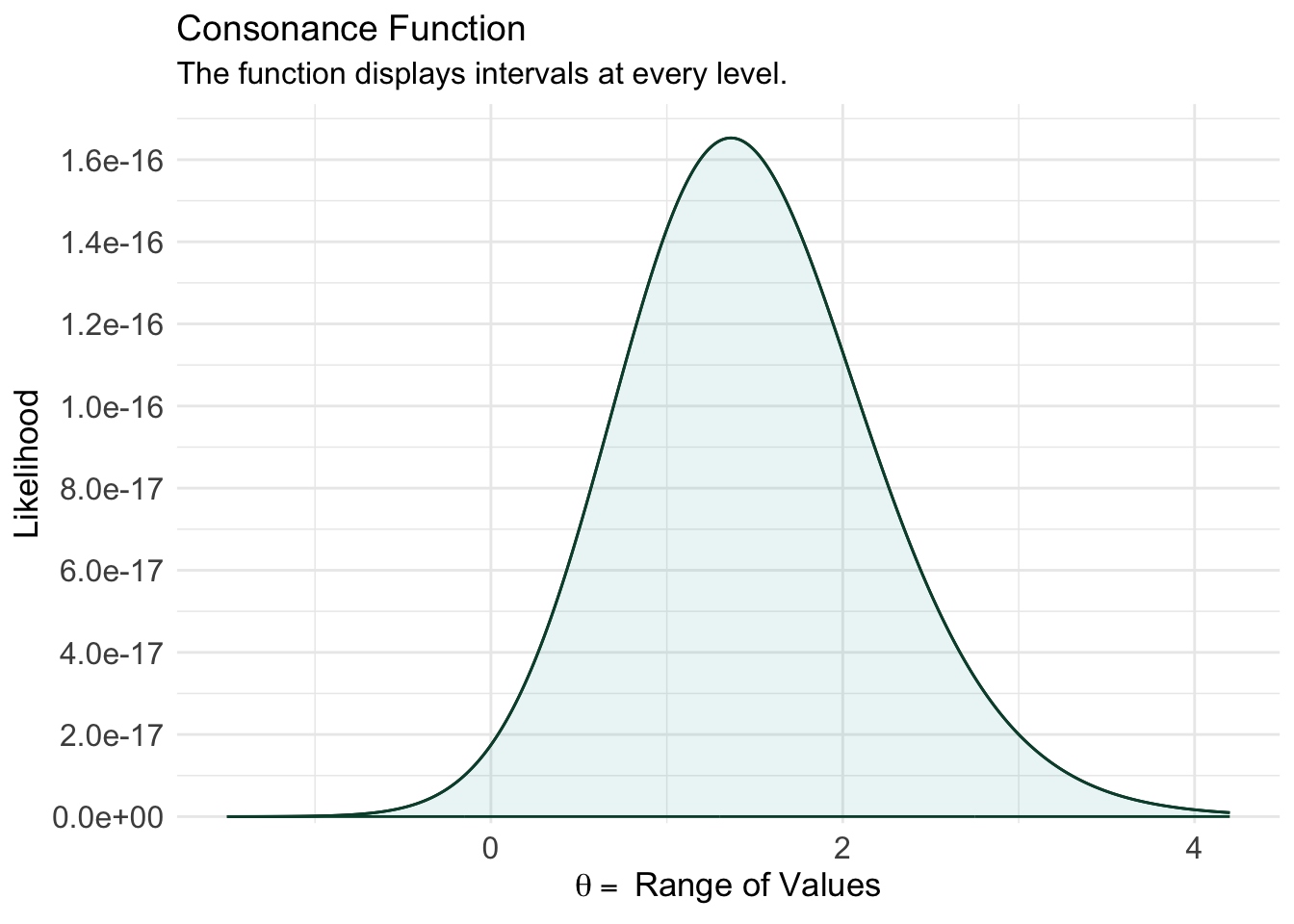
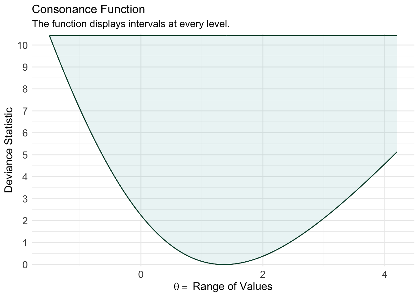
profilelike.glm profiles one coefficient of a GLM over a grid, and curve_lik turns that straight into a concurve object — which then gives all four coordinate views from the top of this post off a single fit. The self-check: the profile’s peak must reproduce the coefficient from the ordinary glm.
library(ProfileLikelihood)
data(dataglm)

xx <- profilelike.glm(y ~ x1 + x2, data = dataglm, profile.theta = "group",
                      lo.theta = -1.5, hi.theta = 4.2,
                      family = binomial(link = "logit"), length = 500, round = 2)
lik_pl <- curve_lik(xx, data = dataglm)

si <- curve_support(lik_pl[[1]], 6.83)
si| k | support.level | lower.limit | upper.limit | mle |
|---|---|---|---|---|
| 6.83 | 0.146 | 0.098 | 2.91 | 1.36 |
# the profile peak must land on the full-model MLE
mod_pl <- glm(y ~ x1 + x2 + group, data = dataglm,
              family = binomial(link = "logit"))
stopifnot(abs(si$mle - coef(mod_pl)[["group"]]) < 0.01)
cat("validation PASSED: profile peak == glm coefficient\n")
#> validation PASSED: profile peak == glm coefficient
The same object, four ways — relative likelihood, log-likelihood, likelihood, and deviance:
Profile versus Wald, and where the 1/6.83 interval lands
curve_lik_glm profiles a coefficient directly. Comparing it against the Wald normal approximation on the same grid shows the skew the Wald interval discards — and the Wald support interval reproduces its own consonance interval, which is the identity from the top of this post:
mod <- glm(am ~ mpg, family = binomial, data = mtcars)
est <- coef(mod)[["mpg"]]
se  <- sqrt(diag(vcov(mod)))[["mpg"]]

lik_prof <- curve_lik_glm(mod, "mpg", steps = 200)
grid     <- lik_prof[[1]]$values
lik_wald <- as_concurve_lik(grid, dnorm(grid, mean = est, sd = se, log = TRUE))

cons <- curve_analytic(estimate = est, se = se, dist = "z")
ci95 <- cons[[1]][which.min(abs(cons[[1]]$intrvl.level - 0.95)),
                  c("lower.limit", "upper.limit")]

out <- rbind(
  `profile 1/6.83 support` = unlist(curve_support(lik_prof[[1]], 6.83)[c("lower.limit", "upper.limit")]),
  `Wald    1/6.83 support` = unlist(curve_support(lik_wald,      6.83)[c("lower.limit", "upper.limit")]),
  `Wald    95% consonance` = unlist(ci95)
)
out
#>                        lower.limit upper.limit
#> profile 1/6.83 support      0.1218       0.588
#> Wald    1/6.83 support      0.0818       0.532
#> Wald    95% consonance      0.0819       0.532

# Wald support interval and Wald consonance interval agree to ~1e-3
stopifnot(max(abs(out[2, ] - out[3, ])) < 1e-3)
cat("validation PASSED: Wald 1/6.83 support == Wald 95% consonance\n")
#> validation PASSED: Wald 1/6.83 support == Wald 95% consonance
The profile curve leans right of the symmetric Wald curve, and that lean is precisely what a Wald interval throws away:
plot_compare(lik_prof[[1]], lik_wald, type = "l1",
             xaxis = expression(beta[mpg]))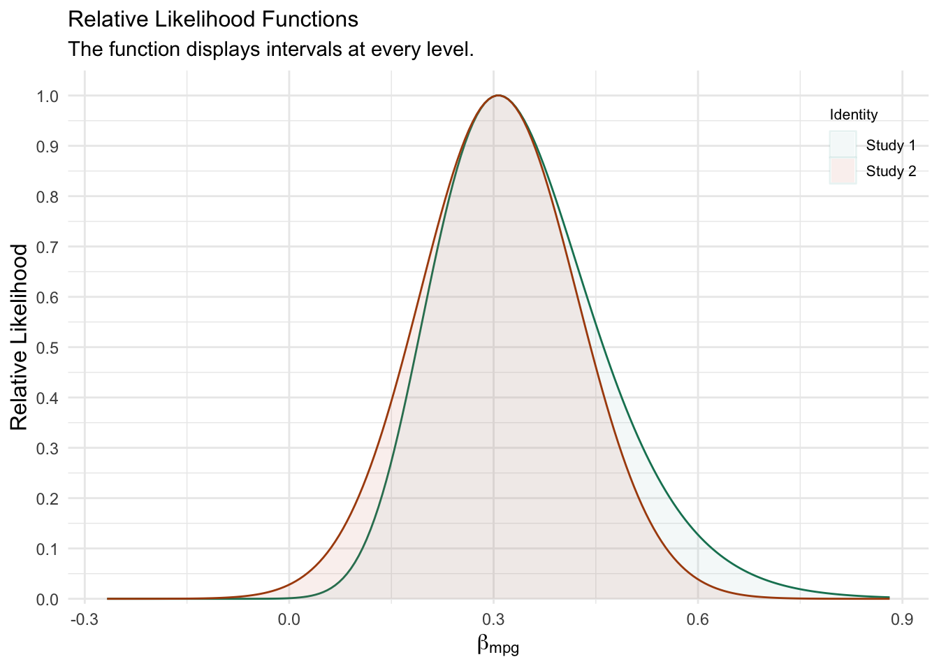
Profile likelihood for a regression coefficient
The offset trick: to fix the coefficient of at , move into an offset and refit the model without . The refit re-maximizes the intercept and the other covariates at every grid point – that is what makes it a profile likelihood rather than a slice through the likelihood at the MLEs.
version 16
clear all
set seed 1031

set obs 300
generate x = rnormal(0, 1)
generate w = rnormal(0, 1)                       // nuisance covariate
generate y = runiform() < invlogit(-0.3 + 0.8*x + 0.4*w)

* full fit: the MLE and Wald SE define the grid
quietly logit y x w
scalar bhat  = _b[x]
scalar sehat = _se[x]

* grid: MLE +/- 4 SEs, 121 points (each point costs one -logit- refit)
local npts  = 121
local blo   = bhat - 4*sehat
local bstep = 8*sehat / (`npts' - 1)

tempname results
tempfile profile
postfile `results' double(beta ll) using "`profile'", replace

forvalues i = 1/`npts' {
    local b = `blo' + (`i' - 1)*`bstep'
    capture drop off
    quietly generate double off = `b'*x
    quietly logit y w, offset(off)
    post `results' (`b') (e(ll))
}
postclose `results'

use "`profile'", clear

* normalize into support / deviance
quietly summarize ll
generate support  = exp(ll - r(max))
generate deviance = -2*(ll - r(max))

* --- validation 1: profile peak sits at the full-model MLE ---
quietly summarize beta if support == 1
display as text _n "profile peak = " as result %9.6f r(mean)  ///
    as text "   full-model MLE = " as result %9.6f bhat
assert abs(r(mean) - bhat) < `bstep'   // within one grid step

* --- validation 2: 1/6.83 support interval ~ Wald 95% CI ---
quietly summarize beta if support >= 1/6.83
display as text "1/6.83 support interval: [" as result %6.4f r(min)   ///
    as text ", " as result %6.4f r(max) as text "]"                    ///
    as text "   Wald 95% CI: [" as result %6.4f bhat - 1.96*sehat      ///
    as text ", " as result %6.4f bhat + 1.96*sehat as text "]"
* profile and Wald agree closely here (smooth likelihood, moderate n);
* they diverge exactly as much as the likelihood is skewed
assert abs(r(min) - (bhat - 1.96*sehat)) < 3*`bstep'
assert abs(r(max) - (bhat + 1.96*sehat)) < 3*`bstep'
display as result "validation PASSED: profile peak and support interval check out"

* --- plots ---
twoway (line support beta),                                            ///
    xline(`=bhat', lpattern(dash) lcolor(gs10))                        ///
    xline(0, lpattern(dot) lcolor(red))                                ///
    yline(0.1464, lcolor(gs12))                                        ///
    title("Profile Likelihood Function for a Logistic Coefficient")    ///
    subtitle("Nuisance parameters re-maximized at each grid point")    ///
    xtitle("Coefficient of x (log-odds scale)")                        ///
    ytitle("Relative Likelihood") name(prof_lik, replace)

twoway (line deviance beta),                                           ///
    xline(`=bhat', lpattern(dash) lcolor(gs10))                        ///
    yline(3.84, lcolor(gs12))                                          ///
    title("Profile Deviance Function")                                 ///
    subtitle("Horizontal line at 3.84; crossings = 95% profile CI")    ///
    xtitle("Coefficient of x (log-odds scale)")                        ///
    ytitle("Profile Deviance") name(prof_dev, replace)

graph combine prof_lik prof_dev, cols(2)
#> Number of observations (_N) was 0, now 300.
#>
#>
#>
#>
#>
#>
#>
#>
#>
#>
#>
#>
#> (file /var/folders/p4/rr9th0593k1_k0bf90vnc57w0000gn/T//S_81055.000001
#>     not found)
#>
#>
#>
#>
#>
#>
#>
#>
#>
#> profile peak =  0.748198   full-model MLE =  0.748198
#>
#>
#>
#> 1/6.83 support interval: [0.4730, 1.0430]   Wald 95% CI: [0.4593, 1.0371]
#>
#>
#>
#> validation PASSED: profile peak and support interval check out
Validation status
| Language | Runtime validated | Notes |
|---|---|---|
| Python | yes – all asserts pass | scipy/statsmodels/matplotlib |
| Julia | yes – all asserts pass (numerics) | Plots.jl output not exercised |
| MATLAB | yes – executes at render via matlab -batch |
fminsearch is base MATLAB; glmfit/normcdf need the Statistics Toolbox |
| SQL (DuckDB, live) | yes – executes at render; asserts vs lm/pnorm |
agreement to machine precision; plotting delegated to R |
| SQL (Snowflake) | yes – all three parts run live there | same logic, dialect differs in row generation |
| Stata | syntax verified against [R] ml, [P] postfile |
run once locally; asserts are the safety net |
Stata cifunction |
asserts against reported CI + z-grid construction | SSC module; conventions per the cifunction guide |
Package Citations
citation("Statamarkdown")
#> To cite package ‘Statamarkdown’ in publications use:
#>
#>   Hemken D, Palmer T (2026). _Statamarkdown: 'Stata' Markdown_. doi:10.32614/CRAN.package.Statamarkdown
#>   <https://doi.org/10.32614/CRAN.package.Statamarkdown>. R package version 1.1.0,
#>   <https://CRAN.R-project.org/package=Statamarkdown>.
#>
#> A BibTeX entry for LaTeX users is
#>
#>   @Manual{,
#>     title = {Statamarkdown: 'Stata' Markdown},
#>     author = {Doug Hemken and Tom Palmer},
#>     year = {2026},
#>     note = {R package version 1.1.0},
#>     url = {https://CRAN.R-project.org/package=Statamarkdown},
#>     doi = {10.32614/CRAN.package.Statamarkdown},
#>   }
citation("reticulate")
#> To cite package ‘reticulate’ in publications use:
#>
#>   Kalinowski T, Ushey K, Allaire J, Tang Y (2026). _reticulate: Interface to 'Python'_.
#>   doi:10.32614/CRAN.package.reticulate <https://doi.org/10.32614/CRAN.package.reticulate>. R package version 1.47.0,
#>   <https://CRAN.R-project.org/package=reticulate>.
#>
#> A BibTeX entry for LaTeX users is
#>
#>   @Manual{,
#>     title = {reticulate: Interface to 'Python'},
#>     author = {Tomasz Kalinowski and Kevin Ushey and JJ Allaire and Yuan Tang},
#>     year = {2026},
#>     note = {R package version 1.47.0},
#>     url = {https://CRAN.R-project.org/package=reticulate},
#>     doi = {10.32614/CRAN.package.reticulate},
#>   }
citation("JuliaCall")
#> To cite package ‘JuliaCall’ in publications use:
#>
#>   Li C (2019). “JuliaCall: an R package for seamless integration between R and Julia.” _The Journal of Open Source
#>   Software_, *4*(35), 1284. doi:10.21105/joss.01284 <https://doi.org/10.21105/joss.01284>.
#>
#> A BibTeX entry for LaTeX users is
#>
#>   @Article{JuliaCall,
#>     author = {Changcheng Li},
#>     title = {{JuliaCall}: an {R} package for seamless integration between {R} and {Julia}},
#>     journal = {The Journal of Open Source Software},
#>     publisher = {The Open Journal},
#>     year = {2019},
#>     volume = {4},
#>     number = {35},
#>     pages = {1284},
#>     doi = {10.21105/joss.01284},
#>   }
Statistical Environments
R Environment
#> ─ Session info ─────────────────────────────────────────────────────────────────────────────────────────────────────────────────
#>  setting  value
#>  version  R version 4.6.1 (2026-06-24)
#>  os       macOS Golden Gate 27.0
#>  system   aarch64, darwin25.4.0
#>  ui       unknown
#>  language (EN)
#>  collate  C.UTF-8
#>  ctype    C.UTF-8
#>  tz       America/New_York
#>  date     2026-09-28
#>  pandoc   3.11 @ /opt/homebrew/bin/ (via rmarkdown)
#>  quarto   1.10.18 @ /usr/local/bin/quarto
#>
#> ─ Packages ─────────────────────────────────────────────────────────────────────────────────────────────────────────────────────
#>  package           * version    date (UTC) lib source
#>  abind               1.4-8      2024-09-12 [1] CRAN (R 4.6.1)
#>  Amelia            * 1.8.3      2024-11-08 [1] CRAN (R 4.6.1)
#>  arm                 1.15-3     2026-04-15 [1] CRAN (R 4.6.1)
#>  arrayhelpers        1.1-2      2026-07-24 [1] CRAN (R 4.6.1)
#>  backports           1.5.1      2026-04-03 [1] CRAN (R 4.6.1)
#>  base              * 4.6.1      2026-06-24 [2] local
#>  base64enc           0.1-6      2026-02-02 [1] CRAN (R 4.6.1)
#>  bayesplot         * 1.16.0     2026-08-25 [1] CRAN (R 4.6.1)
#>  bbmle             * 1.0.26     2026-08-31 [1] CRAN (R 4.6.1)
#>  bdsmatrix           1.3-7      2024-03-02 [1] CRAN (R 4.6.1)
#>  bitops              1.1-0      2026-07-30 [1] CRAN (R 4.6.1)
#>  blogdown          * 1.24       2026-06-19 [1] CRAN (R 4.6.1)
#>  boot              * 1.3-32     2025-08-29 [1] CRAN (R 4.6.1)
#>  bootImpute        * 1.3.0      2025-12-15 [1] CRAN (R 4.6.1)
#>  bridgesampling      1.2-1      2025-11-19 [1] CRAN (R 4.6.1)
#>  brms              * 2.23.0     2025-09-09 [1] CRAN (R 4.6.1)
#>  Brobdingnag         1.3-1      2026-09-12 [1] CRAN (R 4.6.1)
#>  broom             * 1.0.13     2026-05-14 [1] CRAN (R 4.6.1)
#>  broom.mixed       * 0.2.9.7    2026-02-17 [1] CRAN (R 4.6.1)
#>  Cairo             * 1.7-0      2025-10-29 [1] CRAN (R 4.6.1)
#>  car               * 3.1-5      2026-02-03 [1] CRAN (R 4.6.1)
#>  carData           * 3.0-6      2026-01-30 [1] CRAN (R 4.6.1)
#>  caTools             1.18.4     2026-07-20 [1] CRAN (R 4.6.1)
#>  checkmate         * 2.3.4      2026-02-03 [1] CRAN (R 4.6.1)
#>  class               7.3-24     2026-08-03 [1] CRAN (R 4.6.1)
#>  cli               * 3.6.6      2026-04-09 [1] CRAN (R 4.6.1)
#>  clipr               0.8.1      2026-05-25 [1] CRAN (R 4.6.1)
#>  cluster             2.1.8.3    2026-07-30 [1] CRAN (R 4.6.1)
#>  coda              * 0.19-4.1   2024-01-31 [1] CRAN (R 4.6.1)
#>  codetools           0.2-20     2024-03-31 [1] CRAN (R 4.6.0)
#>  colorspace        * 2.1-3      2026-07-12 [1] CRAN (R 4.6.1)
#>  compiler            4.6.1      2026-06-24 [2] local
#>  concurve          * 3.0.5      2026-09-28 [1] local
#>  cond              * 1.2-4      2025-05-25 [1] CRAN (R 4.6.1)
#>  cowplot           * 1.2.0      2025-07-07 [1] CRAN (R 4.6.1)
#>  crayon              1.5.3      2024-06-20 [1] CRAN (R 4.6.1)
#>  curl                8.0.0      2026-08-25 [1] CRAN (R 4.6.1)
#>  data.table          1.18.6.1   2026-08-24 [1] CRAN (R 4.6.1)
#>  datasets          * 4.6.1      2026-06-24 [2] local
#>  DBI               * 1.3.0      2026-02-25 [1] CRAN (R 4.6.1)
#>  DEoptimR            1.2-2      2026-09-25 [1] CRAN (R 4.6.1)
#>  desc                1.4.3      2023-12-10 [1] CRAN (R 4.6.1)
#>  details             0.4.0      2025-02-09 [1] CRAN (R 4.6.0)
#>  dichromat           2.0-1      2026-07-22 [1] CRAN (R 4.6.1)
#>  digest              0.6.39     2025-11-19 [1] CRAN (R 4.6.1)
#>  distributional      0.9.0      2026-09-08 [1] CRAN (R 4.6.1)
#>  doParallel        * 1.0.17     2022-02-07 [1] CRAN (R 4.6.1)
#>  doRNG               1.8.6.3    2026-02-05 [1] CRAN (R 4.6.1)
#>  dplyr             * 1.2.1      2026-04-03 [1] CRAN (R 4.6.1)
#>  duckdb              1.5.5      2026-07-25 [1] CRAN (R 4.6.1)
#>  e1071               1.7-17     2025-12-18 [1] CRAN (R 4.6.1)
#>  emmeans             2.0.4      2026-07-15 [1] CRAN (R 4.6.1)
#>  estimability        2.0.0      2026-06-26 [1] CRAN (R 4.6.1)
#>  evaluate            1.0.5      2025-08-27 [1] CRAN (R 4.6.1)
#>  extremevalues       2.4.1      2024-12-17 [1] CRAN (R 4.6.1)
#>  farver              2.1.2      2024-05-13 [1] CRAN (R 4.6.1)
#>  fastmap             1.2.0      2024-05-15 [1] CRAN (R 4.6.1)
#>  forcats           * 1.0.1      2025-09-25 [1] CRAN (R 4.6.1)
#>  foreach           * 1.5.2      2022-02-02 [1] CRAN (R 4.6.1)
#>  foreign             0.8-91     2026-01-29 [1] CRAN (R 4.6.1)
#>  Formula             1.2-6      2026-08-03 [1] CRAN (R 4.6.1)
#>  fs                  2.1.0      2026-04-18 [1] CRAN (R 4.6.1)
#>  furrr               0.4.0      2026-03-31 [1] CRAN (R 4.6.1)
#>  future            * 1.76.0     2026-09-24 [1] CRAN (R 4.6.1)
#>  future.apply      * 1.20.2     2026-02-20 [1] CRAN (R 4.6.1)
#>  gamlss            * 5.5-0      2025-08-19 [1] CRAN (R 4.6.1)
#>  gamlss.data       * 6.0-7      2025-09-04 [1] CRAN (R 4.6.1)
#>  gamlss.dist       * 6.1-11     2026-09-10 [1] CRAN (R 4.6.1)
#>  generics            0.1.4      2025-05-09 [1] CRAN (R 4.6.1)
#>  ggcorrplot        * 0.3.0      2026-07-24 [1] CRAN (R 4.6.1)
#>  ggdist              3.3.3      2025-04-23 [1] CRAN (R 4.6.1)
#>  ggplot2           * 4.0.3      2026-04-22 [1] CRAN (R 4.6.1)
#>  ggtext            * 0.2.0      2026-08-28 [1] CRAN (R 4.6.1)
#>  glmnet              5.1        2026-09-24 [1] CRAN (R 4.6.1)
#>  globals             0.19.1     2026-03-13 [1] CRAN (R 4.6.1)
#>  glue                1.8.1      2026-04-17 [1] CRAN (R 4.6.1)
#>  graphics          * 4.6.1      2026-06-24 [2] local
#>  grDevices         * 4.6.1      2026-06-24 [2] local
#>  grid              * 4.6.1      2026-06-24 [2] local
#>  gridExtra           2.3.1      2026-06-25 [1] CRAN (R 4.6.1)
#>  gridtext            0.1.6      2026-02-19 [1] CRAN (R 4.6.0)
#>  gtable              0.3.6      2024-10-25 [1] CRAN (R 4.6.1)
#>  gtsummary         * 2.6.1      2026-09-04 [1] CRAN (R 4.6.1)
#>  here              * 1.0.2      2025-09-15 [1] CRAN (R 4.6.1)
#>  Hmisc             * 5.3-0      2026-09-06 [1] CRAN (R 4.6.1)
#>  hms                 1.1.4      2025-10-17 [1] CRAN (R 4.6.1)
#>  htmlTable           2.5.0      2026-04-22 [1] CRAN (R 4.6.1)
#>  htmltools         * 0.5.9      2025-12-04 [1] CRAN (R 4.6.1)
#>  htmlwidgets         1.6.4      2023-12-06 [1] CRAN (R 4.6.1)
#>  httr                1.4.9      2026-09-01 [1] CRAN (R 4.6.1)
#>  ImputeRobust      * 1.3-1      2018-11-30 [1] CRAN (R 4.6.1)
#>  inline              0.3.21     2025-01-09 [1] CRAN (R 4.6.1)
#>  insight             1.5.4      2026-09-05 [1] CRAN (R 4.6.1)
#>  iterators         * 1.0.14     2022-02-05 [1] CRAN (R 4.6.1)
#>  itertools           0.1-3      2014-03-12 [1] CRAN (R 4.6.1)
#>  jomo                2.7-6      2023-04-15 [1] CRAN (R 4.6.1)
#>  jsonlite            2.0.0      2025-03-27 [1] CRAN (R 4.6.1)
#>  JuliaCall           0.17.6     2024-12-07 [1] CRAN (R 4.6.1)
#>  kableExtra        * 1.4.1      2026-07-08 [1] CRAN (R 4.6.1)
#>  knitr             * 1.52       2026-09-06 [1] CRAN (R 4.6.1)
#>  labeling            0.4.3      2023-08-29 [1] CRAN (R 4.6.1)
#>  laeken              0.5.3      2024-01-25 [1] CRAN (R 4.6.1)
#>  latex2exp         * 0.9.8      2026-01-09 [1] CRAN (R 4.6.1)
#>  lattice           * 0.23-1     2026-08-12 [1] CRAN (R 4.6.1)
#>  lifecycle           1.0.5      2026-01-08 [1] CRAN (R 4.6.1)
#>  listenv             1.0.0      2026-06-22 [1] CRAN (R 4.6.1)
#>  lme4                2.0-6      2026-07-16 [1] CRAN (R 4.6.1)
#>  lmtest              0.9-40     2022-03-21 [1] CRAN (R 4.6.1)
#>  loo               * 2.10.1     2026-07-24 [1] CRAN (R 4.6.1)
#>  lubridate         * 1.9.5      2026-02-04 [1] CRAN (R 4.6.1)
#>  magick              2.9.1      2026-02-28 [1] CRAN (R 4.6.1)
#>  magrittr          * 2.0.5      2026-04-04 [1] CRAN (R 4.6.1)
#>  MASS              * 7.3-66     2026-07-15 [1] CRAN (R 4.6.1)
#>  Matrix            * 1.7-6      2026-07-25 [1] CRAN (R 4.6.1)
#>  MatrixModels        0.5-4      2025-03-26 [1] CRAN (R 4.6.1)
#>  matrixStats         1.5.0      2025-01-07 [1] CRAN (R 4.6.1)
#>  maxLik            * 1.5-2.2    2025-12-29 [1] CRAN (R 4.6.0)
#>  mcmc                0.9-8      2023-11-16 [1] CRAN (R 4.6.1)
#>  MCMCpack          * 1.7-1      2024-08-27 [1] CRAN (R 4.6.1)
#>  methods           * 4.6.1      2026-06-24 [2] local
#>  mgcv              * 1.9-4      2025-11-07 [1] CRAN (R 4.6.0)
#>  mi                * 1.3.1      2026-07-28 [1] CRAN (R 4.6.1)
#>  mice              * 3.19.0     2025-12-10 [1] CRAN (R 4.6.1)
#>  miceadds          * 3.20-10    2026-05-28 [1] CRAN (R 4.6.1)
#>  miceFast          * 0.9.1      2026-02-26 [1] CRAN (R 4.6.1)
#>  minqa               1.2.8      2024-08-17 [1] CRAN (R 4.6.1)
#>  miscTools         * 0.6-30     2026-01-20 [1] CRAN (R 4.6.1)
#>  missForest        * 1.6.1      2025-10-26 [1] CRAN (R 4.6.1)
#>  mitml             * 0.4-5      2023-03-08 [1] CRAN (R 4.6.1)
#>  mitools             2.7        2026-08-31 [1] CRAN (R 4.6.1)
#>  multcomp            1.4-32     2026-08-21 [1] CRAN (R 4.6.1)
#>  mvtnorm           * 1.4-2      2026-07-12 [1] CRAN (R 4.6.1)
#>  nlme              * 3.1-171    2026-09-01 [1] CRAN (R 4.6.1)
#>  nloptr              2.2.1      2025-03-17 [1] CRAN (R 4.6.1)
#>  nnet                7.3-21     2026-08-03 [1] CRAN (R 4.6.1)
#>  numDeriv            2016.8-1.1 2019-06-06 [1] CRAN (R 4.6.1)
#>  opdisDownsampling   1.7        2026-09-04 [1] CRAN (R 4.6.1)
#>  otel                0.2.0      2025-08-29 [1] CRAN (R 4.6.1)
#>  pan                 2.0        2026-06-30 [1] CRAN (R 4.6.1)
#>  parallel          * 4.6.1      2026-06-24 [2] local
#>  parallelly        * 1.48.0     2026-06-29 [1] CRAN (R 4.6.1)
#>  pbmcapply         * 1.5.1      2022-04-28 [1] CRAN (R 4.6.1)
#>  performance       * 0.18.2     2026-09-10 [1] CRAN (R 4.6.1)
#>  pillar              1.11.1     2025-09-17 [1] CRAN (R 4.6.1)
#>  pkgbuild            1.4.8      2025-05-26 [1] CRAN (R 4.6.1)
#>  pkgconfig           2.0.3      2019-09-22 [1] CRAN (R 4.6.1)
#>  plyr                1.8.9      2023-10-02 [1] CRAN (R 4.6.1)
#>  png                 0.1-9      2026-03-15 [1] CRAN (R 4.6.0)
#>  polspline           1.1.25     2024-05-10 [1] CRAN (R 4.6.1)
#>  posterior         * 1.7.0      2026-04-01 [1] CRAN (R 4.6.1)
#>  pracma              2.4.6      2025-10-22 [1] CRAN (R 4.6.1)
#>  prettyunits         1.2.0      2023-09-24 [1] CRAN (R 4.6.1)
#>  ProfileLikelihood * 1.3        2023-08-25 [1] CRAN (R 4.6.1)
#>  progress          * 1.2.3      2023-12-06 [1] CRAN (R 4.6.1)
#>  proxy               0.4-29     2025-12-29 [1] CRAN (R 4.6.1)
#>  purrr             * 1.2.2      2026-04-10 [1] CRAN (R 4.6.1)
#>  qqconf              1.3.2      2023-04-14 [1] CRAN (R 4.6.1)
#>  qqplotr           * 0.0.7      2025-09-05 [1] CRAN (R 4.6.1)
#>  quantreg          * 6.1        2025-03-10 [1] CRAN (R 4.6.1)
#>  QuickJSR            1.11.0     2026-08-21 [1] CRAN (R 4.6.1)
#>  R6                  2.6.1      2025-02-15 [1] CRAN (R 4.6.1)
#>  randomForest      * 4.7-1.2    2024-09-22 [1] CRAN (R 4.6.1)
#>  ranger              0.18.0     2026-01-16 [1] CRAN (R 4.6.1)
#>  rbibutils           2.4.1      2026-01-21 [1] CRAN (R 4.6.1)
#>  RColorBrewer        1.1-3      2022-04-03 [1] CRAN (R 4.6.1)
#>  Rcpp              * 1.1.2      2026-07-05 [1] CRAN (R 4.6.1)
#>  RcppParallel        6.2.1      2026-08-27 [1] CRAN (R 4.6.1)
#>  Rdpack              2.6.6      2026-02-08 [1] CRAN (R 4.6.1)
#>  readr             * 2.2.0      2026-02-19 [1] CRAN (R 4.6.1)
#>  reformulas          0.4.4      2026-02-02 [1] CRAN (R 4.6.1)
#>  rematch2            2.1.2      2020-05-01 [1] CRAN (R 4.6.1)
#>  reshape2          * 1.4.5      2025-11-12 [1] CRAN (R 4.6.1)
#>  reticulate        * 1.47.0     2026-09-03 [1] CRAN (R 4.6.1)
#>  rlang               1.3.0      2026-07-05 [1] CRAN (R 4.6.1)
#>  rmarkdown         * 2.32       2026-09-01 [1] CRAN (R 4.6.1)
#>  rms               * 8.1-1      2026-02-18 [1] CRAN (R 4.6.1)
#>  rngtools            1.5.2      2021-09-20 [1] CRAN (R 4.6.1)
#>  robustbase          0.99-7     2026-02-05 [1] CRAN (R 4.6.1)
#>  rpart               4.1.27     2026-03-27 [1] CRAN (R 4.6.0)
#>  rprojroot           2.1.1      2025-08-26 [1] CRAN (R 4.6.1)
#>  rstan             * 2.32.7     2025-03-10 [1] CRAN (R 4.6.1)
#>  rstantools          2.7.1      2026-09-04 [1] Github (stan-dev/rstantools@4d84659)
#>  rstudioapi          0.19.0     2026-06-11 [1] CRAN (R 4.6.1)
#>  S7                  0.2.2      2026-04-22 [1] CRAN (R 4.6.1)
#>  sandwich            3.1-3      2026-08-03 [1] CRAN (R 4.6.1)
#>  scales              1.4.0      2025-04-24 [1] CRAN (R 4.6.1)
#>  sessioninfo         1.2.4      2026-06-04 [1] CRAN (R 4.6.1)
#>  shape               1.4.6.1    2024-02-23 [1] CRAN (R 4.6.1)
#>  showtext          * 0.9-8      2026-03-21 [1] CRAN (R 4.6.1)
#>  showtextdb        * 3.0        2020-06-04 [1] CRAN (R 4.6.1)
#>  sp                  2.2-3      2026-07-19 [1] CRAN (R 4.6.1)
#>  SparseM           * 1.84-2     2024-07-17 [1] CRAN (R 4.6.1)
#>  splines           * 4.6.1      2026-06-24 [2] local
#>  StanHeaders       * 2.39.1     2026-09-02 [1] CRAN (R 4.6.1)
#>  Statamarkdown     * 1.1.0      2026-09-23 [1] CRAN (R 4.6.1)
#>  statmod           * 1.5.2      2026-05-17 [1] CRAN (R 4.6.1)
#>  stats             * 4.6.1      2026-06-24 [2] local
#>  stats4            * 4.6.1      2026-06-24 [2] local
#>  stringi             1.8.9      2026-08-04 [1] CRAN (R 4.6.1)
#>  stringr           * 1.6.0      2025-11-04 [1] CRAN (R 4.6.1)
#>  survival          * 3.8-12     2026-09-09 [1] CRAN (R 4.6.1)
#>  svglite           * 2.2.2      2025-10-21 [1] CRAN (R 4.6.1)
#>  svgPanZoom          0.3.4      2020-02-15 [1] CRAN (R 4.6.1)
#>  svUnit              1.0.8      2025-08-26 [1] CRAN (R 4.6.1)
#>  sysfonts          * 0.8.9      2024-03-02 [1] CRAN (R 4.6.1)
#>  systemfonts         1.3.2      2026-03-05 [1] CRAN (R 4.6.1)
#>  tensorA             0.36.2.1   2023-12-13 [1] CRAN (R 4.6.0)
#>  texPreview        * 2.1.0      2024-01-24 [1] CRAN (R 4.6.0)
#>  textshaping         1.0.5      2026-03-06 [1] CRAN (R 4.6.0)
#>  TH.data             1.1-5      2025-11-17 [1] CRAN (R 4.6.0)
#>  tibble            * 3.3.1      2026-01-11 [1] CRAN (R 4.6.1)
#>  tidybayes         * 3.0.7      2024-09-15 [1] CRAN (R 4.6.1)
#>  tidyr             * 1.3.2      2025-12-19 [1] CRAN (R 4.6.1)
#>  tidyselect          1.2.1      2024-03-11 [1] CRAN (R 4.6.1)
#>  tidyverse         * 2.0.0      2023-02-22 [1] CRAN (R 4.6.1)
#>  timechange          0.4.0      2026-01-29 [1] CRAN (R 4.6.1)
#>  tinytex           * 0.61       2026-09-17 [1] CRAN (R 4.6.1)
#>  tools               4.6.1      2026-06-24 [2] local
#>  twosamples          2.0.1      2023-06-23 [1] CRAN (R 4.6.1)
#>  tzdb                0.5.0      2025-03-15 [1] CRAN (R 4.6.1)
#>  utils             * 4.6.1      2026-06-24 [2] local
#>  V8                  8.2.0      2026-04-21 [1] CRAN (R 4.6.0)
#>  vcd                 1.4-14     2026-07-29 [1] CRAN (R 4.6.1)
#>  vctrs               0.7.3      2026-04-11 [1] CRAN (R 4.6.1)
#>  VIM               * 7.3.1      2026-09-11 [1] CRAN (R 4.6.1)
#>  viridisLite         0.4.3      2026-02-04 [1] CRAN (R 4.6.1)
#>  wesanderson       * 0.3.7      2023-10-31 [1] CRAN (R 4.6.1)
#>  whisker             0.4.1      2022-12-05 [1] CRAN (R 4.6.1)
#>  withr               3.0.3      2026-06-19 [1] CRAN (R 4.6.1)
#>  xfun              * 0.61       2026-09-16 [1] CRAN (R 4.6.1)
#>  xgboost             3.2.1.1    2026-03-18 [1] CRAN (R 4.6.1)
#>  xml2                1.6.0      2026-06-22 [1] CRAN (R 4.6.1)
#>  xtable            * 1.8-8      2026-02-22 [1] CRAN (R 4.6.1)
#>  yaml                2.3.12     2025-12-10 [1] CRAN (R 4.6.1)
#>  yardstick         * 1.4.0      2026-04-07 [1] CRAN (R 4.6.1)
#>  zoo                 1.9-1      2026-09-25 [1] CRAN (R 4.6.1)
#>
#>  [1] /opt/homebrew/lib/R/4.6/site-library
#>  [2] /opt/homebrew/Cellar/r/4.6.1/lib/R/library
#>  * ── Packages attached to the search path.
#>
#> ─ External software ────────────────────────────────────────────────────────────────────────────────────────────────────────────
#>  setting        value
#>  cairo          1.18.4
#>  cairoFT        2.14.3/2.18.1
#>  pango
#>  png
#>  jpeg
#>  tiff
#>  tcl            9.0
#>  curl           8.7.1
#>  zlib           1.2.12
#>  bzlib          1.0.8, 13-Jul-2019
#>  xz             5.8.3
#>  deflate
#>  zstd           1.5.7
#>  PCRE           10.48 2026-08-31
#>  ICU            78.1
#>  TRE            TRE 0.8.0 R_fixes (BSD)
#>  iconv          Apple or GNU libiconv 1.11 /usr/lib/libiconv.2.dylib
#>  readline       8.3
#>  BLAS           /opt/homebrew/Cellar/openblas/0.3.34/lib/libopenblasp-r0.3.34.dylib
#>  lapack         /opt/homebrew/Cellar/r/4.6.1/lib/R/lib/libRlapack.dylib
#>  lapack_version 3.12.1
#>
#> ────────────────────────────────────────────────────────────────────────────────────────────────────────────────────────────────
#> $RNGkind
#> [1] "Mersenne-Twister" "Inversion"        "Rejection"
Stata Environment
set linesize 255
display %tcMonth_dd,CCYY_hh:MM_am now()
about
#>  September 28,2026 8:53 pm
#>
#>
#> StataNow/MP 19.5 for Mac (Apple Silicon)
#> Revision 12 Aug 2026
#> Copyright 1985-2025 StataCorp LLC
#>
#> Total physical memory: 48.01 GB
#>
#> Stata license: Single-user 2-core , expiring  6 Feb 2027
#> Serial number: 501909358563
#>   Licensed to: Zad Rafi
#>
References
References
1. Cole SR, Chu H, Greenland S. (2013). “Maximum likelihood, profile likelihood, and penalized likelihood: A primer.” American Journal of Epidemiology. 179:252–260. doi: 10.1093/aje/kwt245. https://doi.org/10.1093/aje/kwt245.
Abstract
The method of maximum likelihood is widely used in epidemiology, yet many epidemiologists receive little or no education in the conceptual underpinnings of the approach. Here we provide a primer on maximum likelihood and some important extensions which have proven useful in epidemiologic research, and which reveal connections between maximum likelihood and Bayesian methods. For a given data set and probability model, maximum likelihood finds values of the model parameters that give the observed data the highest probability. As with all inferential statistical methods, maximum likelihood is based on an assumed model and cannot account for bias sources that are not controlled by the model or the study design. Maximum likelihood is nonetheless popular, because it is computationally straightforward and intuitive and because maximum likelihood estimators have desirable large-sample properties in the (largely fictitious) case in which the model has been correctly specified. Here, we work through an example to illustrate the mechanics of maximum likelihood estimation and indicate how improvements can be made easily with commercial software …
2. Cox DR. (2006). “Principles of Statistical Inference.” Cambridge University Press.
Abstract
In this definitive book, D. R. Cox gives a comprehensive and balanced appraisal of statistical inference. He develops the key concepts, describing and comparing the main ideas and controversies over foundational issues that have been keenly argued for more than two-hundred years. Continuing a sixty-year career of major contributions to statistical thought, no one is better placed to give this much-needed account of the field. An appendix gives a more personal assessment of the merits of different ideas. The content ranges from the traditional to the contemporary. While specific applications are not treated, the book is strongly motivated by applications across the sciences and associated technologies. The mathematics is kept as elementary as feasible, though previous knowledge of statistics is assumed. The book will be valued by every user or student of statistics who is serious about understanding the uncertainty inherent in conclusions from statistical analyses.
Citation
BibTeX citation:
@online{rafi2026,
  author = {Rafi, Zad and Rafi, Zad},
  title = {Constructing {Likelihood} {Functions} in {R,} {Stata,}
    {Python,} {Julia,} {MATLAB,} and {SQL}},
  date = {2026-09-24},
  url = {https://lesslikely.com/statistics/likelihood-polyglot.html},
  langid = {en-US}
}
Comments