---
title: "How much can six months tell us? NYC comparator methods lab"
subtitle: "Demonstrating robustness checks for cityoutcomes.com with synthetic data"
description: "A synthetic-data demonstration of baseline, weighting, placebo, and trend-sensitivity checks for NYC homicide comparisons."
author: "Kremu"
date: 2026-10-01
categories: [statistics, causal inference, interactive]
image: ../images/HomeLogo-static.webp
bibliography: nyc-comparator/references.bib
csl: custom.csl
format:
html:
toc: true
code-fold: true
code-summary: "Show code"
fig-width: 7
fig-height: 4
execute:
freeze: false
warning: false
message: false
params:
data_path: "nyc-comparator/data/homicides.csv" # city, month, homicides, population
focus: "New York"
event: "2026-01-01"
pre: 12 # baseline months (primary)
n_post: 6 # Jan-Jun 2026
noise_window: 24 # pre months used for RMSPE and slope
start: "2018-01-01"
end: "2026-06-01"
---
```{r setup}
suppressPackageStartupMessages({
  library(dplyr)
  library(ggplot2)
})
source("nyc-comparator/R/rebuttal_funs.R")
source("nyc-comparator/R/simulate_demo.R")
source("nyc-comparator/R/verify_dashboard.R")

DEMO <- !file.exists(params$data_path)
raw  <- if (DEMO) simulate_demo() else read.csv(params$data_path)
d    <- prep_panel(raw) |> balance_panel(params$start, params$end)
verify_dashboard_inputs("nyc-comparator", DEMO, params$start, params$end, params$event, params$focus)

focus <- params$focus
event <- as.Date(params$event)
pre <- params$pre; n_post <- params$n_post
stopifnot(focus %in% d$city)

g_eq  <- gap_series(d, focus, "equal")
g_pop <- gap_series(d, focus, "pop")

nyc_base_rate <- d |>
  filter(city == focus, month < event) |>
  slice_tail(n = pre) |>
  summarise(mean(rate)) |>
  pull()
pct <- function(x) sprintf("%+.0f%%", 100 * x / nyc_base_rate)
pm <- function(x) sprintf("±%.0f%%", abs(100 * x / nyc_base_rate))
f2  <- function(x) sprintf("%.2f", x)
theme_set(theme_minimal(base_size = 11))
```
::: {.callout-warning appearance="simple"}
`r if (DEMO) "**DEMO DATA.** No input file was found at the configured path, so every number below comes from a synthetic panel. These simulated numbers cannot support claims about actual NYC outcomes." else paste0("**Data:** ", params$data_path, " (", n_distinct(d$city), " cities, ", format(min(d$month), "%b %Y"), " to ", format(max(d$month), "%b %Y"), ").")`
The bundled simulation uses seed 2026 and sets NYC's added post-event effect to zero. Shared shocks multiply the cities' different baseline rates, so additive level-gap parallel trends need not hold even without a policy effect. Thus, this demo combines count noise with simulated drift, seasonality and model dependence. It does not measure power to detect an observed policy effect.
:::
Six months is not a lot of data. The [City Outcomes NYC Comparator Lab](https://cityoutcomes.com/) compares New York with a set of peer cities, and its homicide tab (checked October 1, 2026) discloses limited pretrend power and the components of its uncertainty. Here, we'd like to walk through how much the answer from a design like that can move when we change the baseline, the peer weights, or the noise model.
This methods lab adapts material supplied by Kremu. **All bundled results use simulated data**, not observed NYC outcomes. Thus, it evaluates analytical choices, and it says nothing about the effects of Zohran Mamdani's policies. We would need real data, and a reconciliation with that tab, before calling any of this an empirical replication or refutation.
There is also an [interactive dashboard](nyc-comparator-dashboard.qmd) that runs the same estimators. If some of the terms below are unfamiliar, the posts on [S-values](s-values.qmd) and [model assumptions](assumptions.qmd) cover the background.
## What this document does and does not claim
It **does not** claim the new administration changed homicide in either direction.
What it does is show how baseline choices, weighting, placebo comparisons, and assumed drift change an analysis. However, with synthetic inputs, it cannot test the site's empirical conclusion.
## Fixed primary specification
These are the analysis choices that came with the supplied material. No timestamped registration record was included, so we don't claim preregistration here. Still, fixing one specification up front helps us tell the primary calculation apart from the exploratory settings.
| Choice | Value | Why |
|---|---|---|
| Outcome | Monthly homicide rate per 100k | The site's headline tab |
| Event date | `r format(event, "%b %Y")` | Same as the site |
| Post window | `r n_post` months | All available data |
| Primary baseline | Mean of the last `r pre` pre-event months | A single-month baseline is noisy |
| Replication baseline | t−1 only, equal weights | Matches the conventional baseline and weighting rule; real-data replication remains unverified |
| Peer weights | Equal (primary) and population-pooled | The site uses equal |
| Diagnostics | Placebo ranks, three noise summaries and a historical-window sensitivity | One treated unit |
| Sensitivity | Year-over-year seasonal check; linear-drift tipping point | Pretrend power is low |
## 1. Demonstrating the conventional estimator
```{r replicate}
site_est <- did_estimate(g_eq, event, pre, n_post, baseline = "last")
ep <- event_path(g_eq, event) |> filter(rel_month >= -48)
latest <- tail(ep$effect, 1)
```
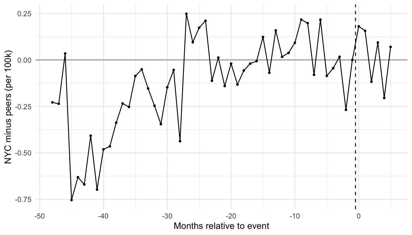
Let's start with the conventional estimator. Using the site's method (equal-weighted peers, rebased to t−1), the mean post-period change in the NYC–peer gap relative to December 2025 is **`r f2(site_est)`** per 100k/month. The latest single-month gap change is **`r f2(latest)`**.
`r if (!DEMO) "Compare against the value the site publishes for the latest month. If the two don't match, stop and reconcile before reading further." else ""`
```{r fig-event}
#| fig-alt: "Synthetic focal-city minus peer-rate changes relative to December 2025."
#| fig-cap: "Synthetic event-study path (rebased so t−1 = 0)."
ggplot(ep, aes(rel_month, effect)) +
  geom_hline(yintercept = 0, colour = "grey60") +
  geom_vline(xintercept = -0.5, linetype = 2) +
  geom_line() + geom_point(size = 0.8) +
  labs(x = "Months relative to event", y = "NYC minus peers (per 100k)")
```
## 2. The point estimate depends on unforced choices
```{r variants}
variants <- tibble::tibble(
  Specification = c("Site: t-1 baseline, equal weights",
                    "12-month mean baseline, equal weights (primary)",
                    "12-month mean baseline, population weights",
                    "6-month mean baseline, equal weights",
                    "24-month mean baseline, equal weights",
                    "Year-over-year, same months (seasonality-robust)"),
  Estimate = c(site_est,
               did_estimate(g_eq,  event, 12, n_post),
               did_estimate(g_pop, event, 12, n_post),
               did_estimate(g_eq,  event, 6,  n_post),
               did_estimate(g_eq,  event, 24, n_post),
               yoy_estimate(g_eq, event, n_post))
) |> mutate(`% of NYC baseline` = pct(Estimate))
knitr::kable(variants |> mutate(Estimate = f2(Estimate)))
primary <- did_estimate(g_eq, event, pre, n_post)
```
NYC's baseline rate is **`r f2(nyc_base_rate)`** per 100k per month. As we can see from the table, the estimate depends on choices that nothing forces on us. That spread across defensible specifications is itself a form of uncertainty, and the illustrative intervals below condition on whichever specification was chosen.
A note on the percentage column. It divides the estimated change in the NYC–peer gap by NYC's 12-month baseline rate, so it should not be read as NYC's own percentage rate change (both NYC and peer rates enter the contrast). Thus, a value below −100% can occur even when every homicide rate is nonnegative.
## 3. How big an effect could six months detect?
With a single treated unit, the variance model does most of the work. The site's methodology, checked October 1, 2026, discloses cross-peer variation, Poisson count variance, and Newey–West slope uncertainty. We don't reproduce its full interval calculation here. Instead, here's a table of three illustrative noise summaries and a historical-window sensitivity:
```{r precision}
fake <- seq(as.Date("2019-01-01"), as.Date("2025-01-01"), by = "year")
itp  <- in_time_placebos(g_eq, fake, pre, n_post)
isp  <- in_space_placebos(d, event, pre, n_post, params$noise_window)
n_itp <- sum(!is.na(itp$estimate))

se_tbl <- tibble::tibble(
  `Variance model` = c("Focal count-only component (independent Poisson reference)",
                       "NYC's own in-time placebos",
                       "Cross-city placebo spread (alternative diagnostic)",
                       "Own history omitting 2020–2023 events (sensitivity)"),
  SE = c(poisson_se(d, focus, event, pre, n_post),
         sd(itp$estimate, na.rm = TRUE),
         sd(isp$estimate[isp$city != focus], na.rm = TRUE),
         sd(itp$estimate[format(itp$fake_event, "%Y") %in% c("2019", "2024", "2025")], na.rm = TRUE))
) |>
  mutate(`Normal reference band (±1.96 × summary)` = sprintf("%s to %s", f2(primary - 1.96 * SE), f2(primary + 1.96 * SE)),
         `MDE (80% power)` = f2(mde(SE)),
         `MDE as % of NYC baseline` = pm(mde(SE)))
knitr::kable(se_tbl |> mutate(SE = f2(SE)))
```
The minimum detectable effect (MDE) shown here is a normal-approximation planning calculation for 80% power at a two-sided 5% threshold, conditional on the chosen standard error and model. Smaller effects would be detected less often. However, these approximate summaries do not establish the actual power of the site's design.
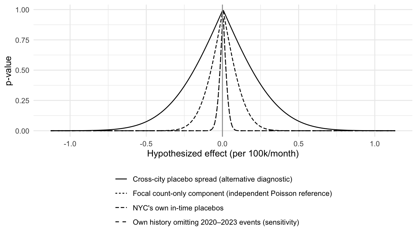
These summaries measure different sources of variation. The count-only component excludes peer counts and dependence. The in-time spread includes count variation and historical change, while the cross-city spread also includes differences between cities. Thus, we treat the bands as descriptive normal references (±1.96 times each summary), without demonstrated 95% coverage. The sensitivity row uses only the 2019, 2024 and 2025 events. It exposes the consequence of omitting 2020–2023 events, but does not establish that three draws provide a better reference. Choosing that summary also changes the approximate MDE and compatibility curve.
Differences in city size can create heteroskedasticity and distort inference with few treated groups [@ferman2019]. That said, this synthetic example does not establish that the site's intervals overstate NYC uncertainty. The in-time placebos use NYC's own history, which seems like the most relevant reference, but there are only `r n_itp` draws, so we should treat that SE as rough. The intervals above also use the normal multiplier 1.96. An illustrative *t* reference with `r n_itp - 1` degrees of freedom and the same SD would use `r sprintf("%.2f", qt(0.975, n_itp - 1))` instead, which widens the in-time interval by about `r sprintf("%.0f", 100 * (qt(0.975, n_itp - 1) / qnorm(0.975) - 1))`%. The placebo windows overlap from one year to the next as well, so the draws are not independent, and the *t* reference should not be taken as a validated correction.
## 4. Which effect sizes are compatible with the data?
```{r svalues}
se_mid <- se_tbl$SE[2]
hyp <- nyc_base_rate * c(-0.5, -0.25, 0, 0.25, 0.5)
sv <- s_values(primary, se_mid, hyp) |>
  mutate(`Hypothesized change` = pct(hypothesis),
         p = sprintf("%.2f", p), `S-value (bits)` = sprintf("%.1f", s_bits)) |>
  select(`Hypothesized change`, p, `S-value (bits)`)
knitr::kable(sv)
```
The table uses NYC's in-time SE. An S-value of *s* bits is about as surprising as seeing *s* heads in a row from a fair coin (the [S-values post](s-values.qmd) goes through this in detail). An S-value below 2 bits corresponds to a *P*-value above 0.25 under the stated normal model. It is NOT the probability that a hypothesis is true.
```{r fig-curve}
#| fig-alt: "Compatibility curves under four illustrative noise summaries, including a historical-window sensitivity."
#| fig-cap: "P-value (compatibility) function for the primary estimate under each variance model."
grid <- seq(primary - 4 * max(se_tbl$SE), primary + 4 * max(se_tbl$SE), length.out = 400)
curves <- lapply(seq_len(nrow(se_tbl)), function(i)
  data.frame(model = se_tbl$`Variance model`[i], h = grid,
             p = s_values(primary, se_tbl$SE[i], grid)$p)) |> bind_rows()
ggplot(curves, aes(h, p, linetype = model)) +
  geom_line() + geom_vline(xintercept = 0, colour = "grey60") +
  labs(x = "Hypothesized effect (per 100k/month)", y = "p-value", linetype = NULL) +
  theme(legend.position = "bottom", legend.direction = "vertical")
```
## 5. Is NYC unusual among its peers? (in-space permutation)
```{r perm}
nyc_row  <- isp |> filter(city == focus)
p_ratio  <- perm_p(isp$ratio, nyc_row$ratio)
p_est    <- perm_p(isp$estimate / isp$pre_rmspe, nyc_row$estimate / nyc_row$pre_rmspe)
rank_r   <- rank(-replace(isp$ratio, !is.finite(isp$ratio), NA_real_), ties.method = "min", na.last = "keep")[isp$city == focus]
```
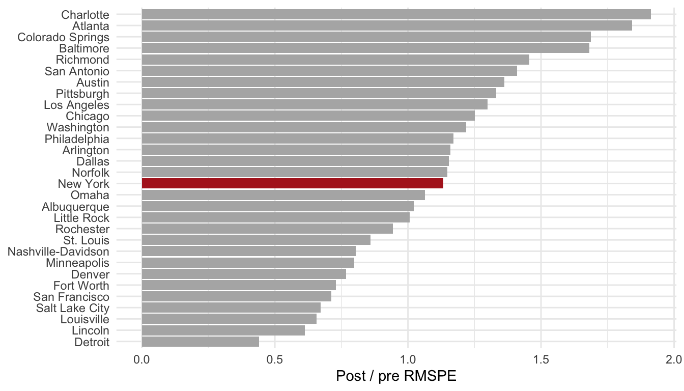
Each city takes a turn as the focus against all other cities, so NYC remains in a peer city's comparator pool. Both RMSPE windows use that city's pre-baseline mean as their center, with a `r params$noise_window`-month pre noise window. We retain this descriptive leave-one-out diagnostic, but a real treatment effect could also enter placebo comparator pools.
Among `r sum(is.finite(isp$ratio))` finite ratios, NYC ranks **`r rank_r`**. The upper-tail ratio share is **`r sprintf("%.2f", p_ratio)`**, and the two-sided share for the standardized estimate is **`r sprintf("%.2f", p_est)`**. The ratio share has a floor of 1/`r sum(is.finite(isp$ratio))` when the focal ratio is finite and included. These are descriptive rankings, which are a long way from a fitted synthetic-control or calibrated randomization analysis.
```{r fig-perm}
#| fig-alt: "Synthetic cities ranked by post-period to pre-period RMSPE ratio."
#| fig-cap: "Post/pre RMSPE ratio for every city treated as the focus."
ggplot(isp, aes(reorder(city, ratio), ratio, fill = city == focus)) +
  geom_col() + coord_flip() +
  scale_fill_manual(values = c("grey70", "firebrick"), guide = "none") +
  labs(x = NULL, y = "Post / pre RMSPE")
```
## 6. Is January 2026 unusual in NYC's own history? (in-time placebos)
```{r fig-itp}
#| fig-alt: "Synthetic estimates at January placebo dates and the analysis date."
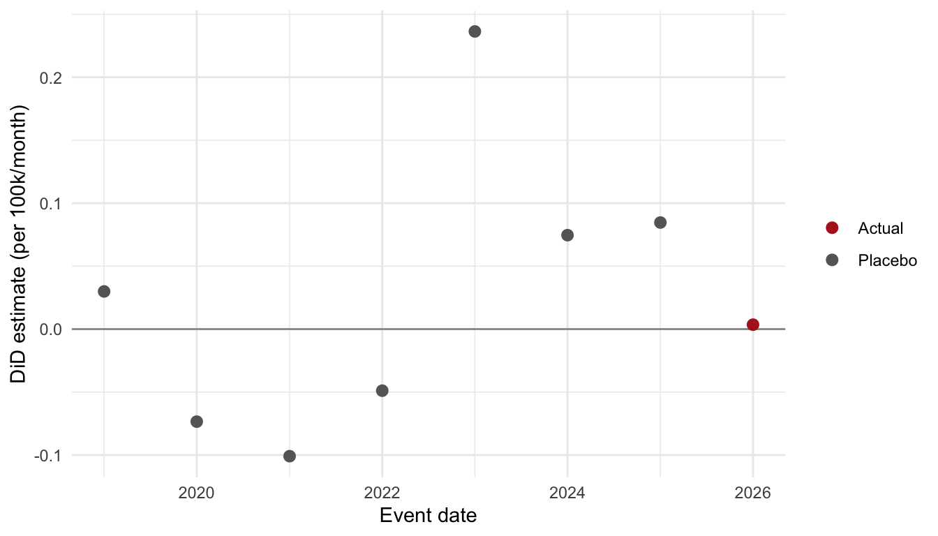
#| fig-cap: "NYC estimate at fake January event dates vs the real one."
itp_plot <- bind_rows(itp |> mutate(type = "Placebo"),
                      tibble::tibble(fake_event = event, estimate = primary, type = "Actual"))
ggplot(itp_plot, aes(fake_event, estimate, colour = type)) +
  geom_hline(yintercept = 0, colour = "grey60") +
  geom_point(size = 2.5) +
  scale_colour_manual(values = c(Actual = "firebrick", Placebo = "grey40")) +
  labs(x = "Event date", y = "DiD estimate (per 100k/month)", colour = NULL)
p_time <- perm_p(c(itp$estimate, primary), primary)
```
Across `r sum(is.finite(c(itp$estimate, primary)))` January start dates (the analysis date included), the share with an estimate at least as large in magnitude as the analysis-date estimate is **`r sprintf("%.2f", p_time)`**. Missing-window estimates are excluded from both the share and its denominator. However, the 2020–2023 event windows include simulated pandemic-era shocks, so the sensitivity row above shows the spread after omitting them. The 2025 placebo's post window also overlaps the primary baseline, making these draws dependent.
## 7. How much trend violation would flip the reading?
```{r trend}
sl  <- pre_slope(g_eq, event, params$noise_window)
lag <- trend_lag(pre, n_post)
delta_grid <- seq(-3, 3, length.out = 121) * max(abs(sl["slope"]), sl["se"])
adj <- drift_adjust(primary, se_mid, delta_grid, lag)
breakdown <- primary / lag
```
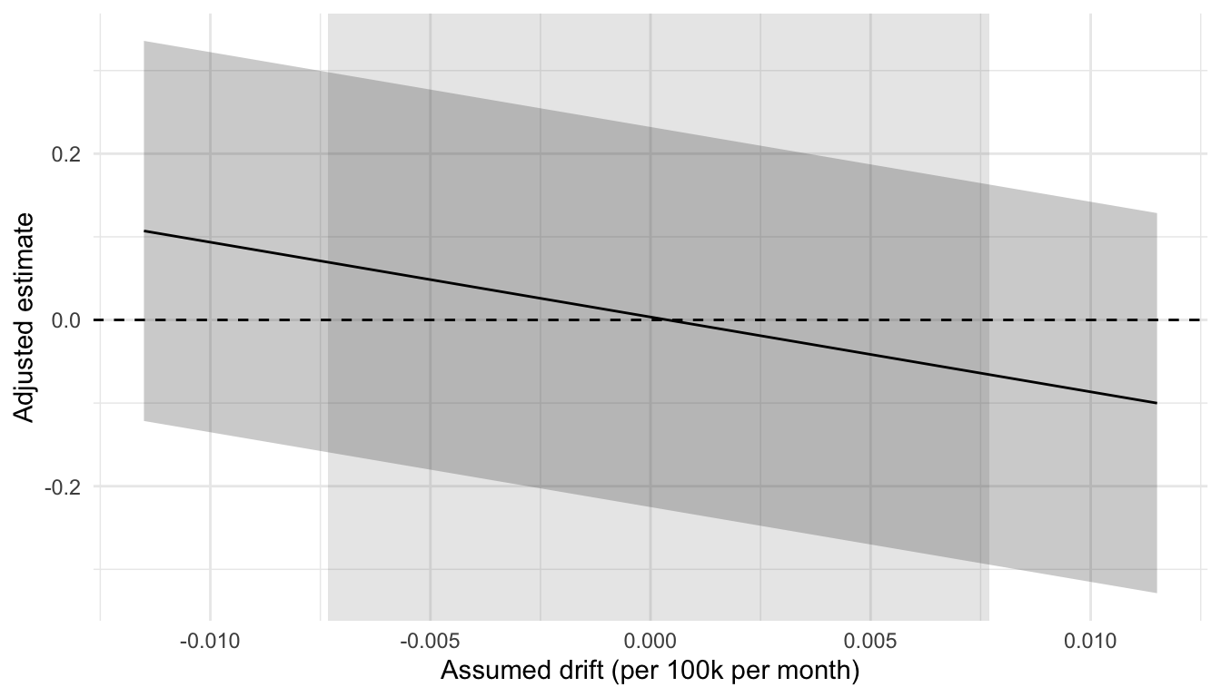
The pre-period slope of the gap is **`r sprintf("%.4f", sl["slope"])`** per month (naive OLS SE `r sprintf("%.4f", sl["se"])`; its ±1.96 × SE reference runs from `r sprintf("%.4f", sl["slope"] - 1.96*sl["se"])` to `r sprintf("%.4f", sl["slope"] + 1.96*sl["se"])`), and the baseline and post midpoints are `r lag` months apart. This reference ignores serial correlation and has no demonstrated coverage. Thus, a differential drift of just **`r sprintf("%.4f", breakdown)`** per month would fully account for the point estimate.
```{r fig-trend}
#| fig-alt: "Adjusted synthetic estimate and interval across assumed linear drifts."
#| fig-cap: "Estimate after removing an assumed linear differential drift. Shaded: naive OLS slope reference (±1.96 SE), ignoring serial correlation."
ggplot(adj, aes(delta, estimate)) +
  annotate("rect", xmin = sl["slope"] - 1.96 * sl["se"], xmax = sl["slope"] + 1.96 * sl["se"],
           ymin = -Inf, ymax = Inf, alpha = 0.15) +
  geom_ribbon(aes(ymin = lo, ymax = hi), alpha = 0.25) +
  geom_line() + geom_hline(yintercept = 0, linetype = 2) +
  labs(x = "Assumed drift (per 100k per month)", y = "Adjusted estimate")
```
This is a linear drift scenario, motivated by work on sensitivity to parallel-trend violations [@rambachan2023]. It does not implement `HonestDiD`, and it does not propagate uncertainty in the assumed drift.
## 8. Scorecard
```{r scorecard}
tibble::tibble(
  Check = c("Conventional estimator", "Specification spread (six report choices)", "Approximate MDE (in-time summary)",
            "Permutation rank", "In-time rank", "Drift breakdown"),
  Result = c(f2(site_est),
             sprintf("%s to %s", f2(min(variants$Estimate, na.rm = TRUE)),
                     f2(max(variants$Estimate, na.rm = TRUE))),
             pm(mde(se_mid)),
             sprintf("%d / %d (tail share = %.2f)", rank_r, sum(is.finite(isp$ratio)), p_ratio),
             sprintf("p = %.2f", p_time),
             sprintf("%.4f per month", breakdown))
) |> knitr::kable()
```
## Limitations of this methods demonstration
- We were not given a real homicide input file or a preregistration record. Thus, no empirical replication or policy-effect conclusion has been established.
- Placebo ranks require exchangeability to be interpreted as calibrated *P*-values. Cities and historical dates are not randomly assigned, so we treat these ranks as descriptive diagnostics. The normal intervals and MDEs condition on illustrative variance models.
- We only cover homicide. Other outcomes would need separate checks of their measurement, geography, timing and comparator definitions.
- Council on Criminal Justice (CCJ) mid-year data are preliminary and subject to revision, so it's worth recording the date the data were pulled.
- The permutation p has a floor of 1/N. The in-time placebos have few draws.
- The linear-drift calculation is illustrative and does not implement HonestDiD robust inference.
As a rule, we'd look to the whole specification table and the interval estimates before any single point estimate, and we'd hold off on any reading of the real site until the real data have been run through the same checks.
## References
::: {#refs}
:::
Comments