
sysuse auto2
#> (1978 automobile data)Using Stata: Producing Consonance Functions
A simple guide on how to produce consonance functions in Stata.
Keywords
Stata, consonance functions, confidence intervals, statistical software, sensitivity analysis, uncertainty analysis, statistical workflow
Although concurve was originally designed to be used in R, it is possible to achieve very similar results in Stata. We can use some datasets that are built into Stata to show how to achieve this. I’ll use the Statamarkdown R package so that I can obtain Stata outputs using RMarkdown via my Stata 16 package.
First, let’s load the auto2 dataset which contains data about cars and their characteristics.
Browse the data set in your data browser to get more familiar with some of the variables. Let’s say we’re interested in the relationship between miles per gallon and price. We could fit a very simple linear model to assess that relationship.
First, let’s visualize the data with a scatter plot.

That’s what our data looks like. Clearly there seems to be an inverse relationship between miles per gallon and price.
Now we could fit a very simple linear model with miles per gallon being the predictor and price being the outcome and get some estimates of the relationship.
sysuse auto2
regress price mpg
#> (1978 automobile data)
#>
#>
#>       Source |       SS           df       MS      Number of obs   =        74
#> -------------+----------------------------------   F(1, 72)        =     20.26
#>        Model |   139449474         1   139449474   Prob > F        =    0.0000
#>     Residual |   495615923        72  6883554.48   R-squared       =    0.2196
#> -------------+----------------------------------   Adj R-squared   =    0.2087
#>        Total |   635065396        73  8699525.97   Root MSE        =    2623.7
#>
#> ------------------------------------------------------------------------------
#>        price | Coefficient  Std. err.      t    P>|t|     [95% conf. interval]
#> -------------+----------------------------------------------------------------
#>          mpg |  -238.8943   53.07669    -4.50   0.000    -344.7008   -133.0879
#>        _cons |   11253.06   1170.813     9.61   0.000     8919.088    13587.03
#> ------------------------------------------------------------------------------
That’s what our output looks like.
Our output also gives us 95% consonance (confidence) intervals by default. But suppose we wished to fit a fractional polynomial model and graph it and get the confidence bands, here’s what we would do.
sysuse auto2
mfp: glm price mpg
twoway (fpfitci price mpg, estcmd(glm) fcolor(dkorange%20) alcolor(%40))  || scatter price mpg, mcolor(dkorange) scale(0.75)
graph export "mfp.svg", replace
#> (1978 automobile data)
#>
#>
#> Deviance for model with all terms untransformed = 1373.079, 74 observations
#>
#> Variable     Model (vs.)   Deviance  Dev diff.   P      Powers   (vs.)
#> ----------------------------------------------------------------------
#> mpg          Lin.   FP2    1373.079    19.565  0.000+   1         -2 -2
#>              FP1           1356.927     3.413  0.182    -2
#>              Final         1356.927                     -2
#>
#>
#> Transformations of covariates:
#>
#> -> gen double Impg__1 = X^-2-.2204707671 if e(sample)
#>    (where: X = mpg/10)
#>
#> Final multivariable fractional polynomial model for price
#> --------------------------------------------------------------------
#>     Variable |    -----Initial-----          -----Final-----
#>              |   df     Select   Alpha    Status    df    Powers
#> -------------+------------------------------------------------------
#>          mpg |    4     1.0000   0.0500     in      2     -2
#> --------------------------------------------------------------------
#>
#> Generalized linear models                         Number of obs   =         74
#> Optimization     : ML                             Residual df     =         72
#>                                                   Scale parameter =    5533697
#> Deviance         =  398426217.4                   (1/df) Deviance =    5533697
#> Pearson          =  398426217.4                   (1/df) Pearson  =    5533697
#>
#> Variance function: V(u) = 1                       [Gaussian]
#> Link function    : g(u) = u                       [Identity]
#>
#>                                                   AIC             =    18.3909
#> Log likelihood   = -678.4632599                   BIC             =   3.98e+08
#>
#> ------------------------------------------------------------------------------
#>              |                 OIM
#>        price | Coefficient  std. err.      z    P>|z|     [95% conf. interval]
#> -------------+----------------------------------------------------------------
#>      Impg__1 |   13163.85   2013.016     6.54   0.000      9218.41    17109.29
#>        _cons |   5538.395   289.7737    19.11   0.000     4970.449    6106.341
#> ------------------------------------------------------------------------------
#> Deviance = 1356.927.
#>
#>
#> file mfp.svg saved as SVG format
That’s what our model looks graphed.

Now suppose we got a single estimate (point or interval) for a parameter, and we wanted all the intervals for it at every level.
Here’s the code that we’ll be using to achieve that in Stata.
#> no; dataset in memory has changed since last saved
#> r(4);
#>
#> r(4);
That’s a lot and may seem intimidating at first, but I’ll explain it line by line.
postfile topost level pvalue svalue lointerval upinterval using my_new_data, replace
#> no; dataset in memory has changed since last saved
#> r(4);“postfile” is the command that will be responsible for pasting the data from our overall loop into a new dataset. Here, we are telling Stata that the internal Stata memory used to hold these results (the post) will be named “topost” and that it will have five variables, “level”, “pvalue”, “svalue”, “lointerval”, and “upinterval.”
“level” will contain the consonance level that corresponds to the limits of the interval, with “lointerval” being the lower bound of the interval and “upinterval” being the upper bound.
“pvalue”is computed by taking 1 - “level”, which is alpha.
“svalue”is computed by taking the of the computed P-value, and this column will be used to plot the surprisal function.
“my_new_data” is the filename that we’ve assigned to our new dataset.
“replace” indicates that if there is an existing filename that already exists, we’re willing to relace it.
Here are the next few major lines
#> no; dataset in memory has changed since last saved
#> r(4);
#>
#>
#> post topost not found
#> r(111);
#>
#> r(111);
The command “forvalues” is responsible for taking a set of numbers that we provide it, and running the contents within the braces through those numbers. So here, we’ve set the local macro “i” to contain numbers between 10 and 99.99 for our consonance levels. Why 10? Stata cannot compute consonance intervals lower than 10%.
Our next line contains the actual contents of what we want to do. Here, it says that we will run a simple linear regression where mpg is the predictor and where price is the outcome, and that the outputs for each loop will be suppressed, hence the “quiet.”
Then, we have the command “level” with the local macro “i” inside of it. As you may already know, “level” dictates the consonance level that Stata provides us. By default, this is set to 95%, but here, we’ve set it “i”, which we established via “forvalues” as being set to numbers between 10 and 99.
The next line two lines
#> no; dataset in memory has changed since last saved
#> r(4);
indicate that we will take variables of a certain class r(), (this class contains the interval bounds we need) and place them within a matrix called E. Then we will list the contents of this matrix.
post topost (`i') (1-`i'/100) ( ln(1-`i'/100)/ln(2) * -1) (E[5,1]) (E[6,1])
#> no; dataset in memory has changed since last saved
#> r(4);
#>
#>
#> post topost not found
#> r(111);
#>
#> r(111);
From the contents of this matrix list, we will take the estimates from the fifth and sixth rows (look at the last two paranthesis of this line of code above and then the image below) in the first column which contain our consonance limits, with the fifth row containing the lower bound of the interval and the sixth containing the upper bound.


We will place the contents from the fifth row into the second variable we set originally for our new dataset, which was “lointerval.” The contents of the sixth row will be placed into “upinterval.”
All potential values of “i” (10-99) will be placed into the first variable that we set, “level”. From this first variable, we can compute the second variable we set up, which was “Pvalue” and we’ve done that here by subtracting “level” from 1 and then dividing the whole equation by 100, so that our P-value can be on the proper scale. Our third variable, which is the longest, computes the “Svalue” by using the previous variable, the “Pvalue” and taking the of it.
The relationships between the variables on this line and the variables we set up in the very first line are dictated by the order of the commands we have set, and therefore they correspond to the same order.
“post topost” is writing the results from each loop as new observations in this data structure.
With that, our loop has concluded, and we can now tell Stata that “post” is no longer needed
postclose topost
#> no; dataset in memory has changed since last saved
#> r(4);
#>
#>
#> post topost not found
#> r(111);
#>
#> r(111);
We then tell Stata to clear its memory to make room for the new dataset we just created and we can list the contents of this new dataset.
Now we have an actual dataset with all the consonance intervals at all the levels we wanted, ranging from 10% all the way up to 99%.
In order to get a function, we’ll need to be able to graph these results, and that can be tricky since for each observation we have one y value (the consonance level), and two x values, the lower bound of the interval and the upper bound of the interval.
So a typical scatterplot will not work, since Stata will only accept one x value. To bypass this, we’ll have to use a paired-coordinate scatterplot which will allow us to plot two different y variables and two different x variables.
Of course, we don’t need two y variables, so we can set both options to the variable “level”, and then we can set our first x variable to “lointerval” and the second x variable to “upinterval.”
This can all be done with the following commands, which will also allow us to set the title and subtitle of the graph, along with the titles of the axes.
twoway (pcscatter level lointerval level upinterval), ///
ytitle(Consonance Level (%)) xtitle(Consonance Limits) ///
title(Consonance Curve) ///
subtitle(A function comprised of several consonance intervals at various levels.)
#> no; dataset in memory has changed since last saved
#> r(4);
#>
#>
#> variable level not found
#> r(111);
#>
#> r(111);
However, I would recommend using the menu to customize the plots as much as possible. Simply go to the Graphics menu and select Twoway Graphs. Then create a new plot definition, and select the Advanced plots and choose a paired coordinate scatterplot and fill in the y variables, both of which will be “levels” and the x variables, which will be “lointerval” and “upinterval”.
So now, here’s what our confidence/consonance function looks like.
clear
sysuse auto2
postfile topost level pvalue svalue lointerval upinterval using my_new_data, replace

forvalues i = 10/99.9 {
      quietly regress price weight, level(`i')
      matrix E = r(table)
      quietly matrix list E
      post topost (`i') (1-`i'/100) ( ln(1-`i'/100)/ln(2) * -1) (E[5,1]) (E[6,1])
    }

postclose topost
use my_new_data, clear

twoway (pcscatter pvalue lointerval pvalue upinterval, mcolor(maroon)), ytitle(Consonance Level (%)) xtitle(Consonance Limits) scale(0.75) ///
title(Consonance Curve) subtitle(A function comprised of several consonance intervals at various levels.)
graph export "confidence.svg", replace
#> no; dataset in memory has changed since last saved
#> r(4);
#>
#>
#>
#> (1978 automobile data)
#>
#>
#>
#>
#>
#>
#> file confidence.svg saved as SVG format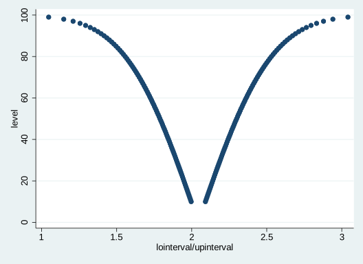
Pretty neat, eh? And below is what our surprisal function looks like, which is simply the (p) transformation of the observed P-value. For a more comprehensive discussion on surprisals, see this page and check out some of the references at the bottom.
clear
sysuse auto2
postfile topost level pvalue svalue lointerval upinterval using my_new_data, replace

forvalues i = 10/99.9 {
      quietly regress price weight, level(`i')
      matrix E = r(table)
      quietly matrix list E
      post topost (`i') (1-`i'/100) ( ln(1-`i'/100)/ln(2) * -1) (E[5,1]) (E[6,1])
    }

postclose topost
use my_new_data, clear

twoway (pcscatter svalue lointerval svalue upinterval, mcolor(maroon)), ytitle(Consonance Level (%)) xtitle(Consonance Limits)  scale( 0.75) ///
title(Surprisal Curve) subtitle(A function comprised of several consonance intervals at various levels.)
graph export "surprisal.svg", replace
#> no; dataset in memory has changed since last saved
#> r(4);
#>
#>
#>
#> (1978 automobile data)
#>
#>
#>
#>
#>
#>
#> file surprisal.svg saved as SVG format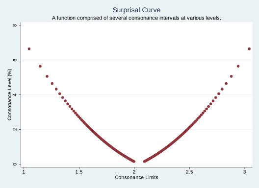
It’s clear that in both plots, we’re missing values of intervals with a confidence/consonance level of less than 10%, but unfortunately, this is the best Stata can do, and what we’ll have to work with. It may not look as pretty as an output from R, but it’s far more useful than blankly staring at a 95% interval and thinking that it is the only piece of information we have regarding compatibility of different effect estimates.
The code that I have pasted above can be used for most commands in Stata that have an option to calculate a consonance level. Thus, if there’s an option for “level”, then the commands above will work to produce a data set of several consonance intervals. Though I am seriously hoping that a Stata expert will see this post and point out how I am wrong.
Now, suppose we wished to fit a generalized linear model, here’s what our code would look like.
#> no; dataset in memory has changed since last saved
#> r(4);
#>
#>
#>
#> (1978 automobile data)
#>
#>
#>
#>
#>
#>
#>      +---------------------------------------------------+
#>      | level   pvalue     svalue   lointer~l   upinter~l |
#>      |---------------------------------------------------|
#>   1. |    10       .9   .1520031    -245.564   -232.2247 |
#>   2. |    11      .89   .1681228   -246.2351   -231.5536 |
#>   3. |    12      .88   .1844246   -246.9073   -230.8814 |
#>   4. |    13      .87   .2009127   -247.5808   -230.2079 |
#>   5. |    14      .86   .2175914   -248.2557    -229.533 |
#>      |---------------------------------------------------|
#>   6. |    15      .85   .2344653   -248.9321   -228.8566 |
#>   7. |    16      .84   .2515388   -249.6102   -228.1785 |
#>   8. |    17      .83   .2688168     -250.29   -227.4987 |
#>   9. |    18      .82   .2863042   -250.9717    -226.817 |
#>  10. |    19      .81   .3040062   -251.6554   -226.1333 |
#>      |---------------------------------------------------|
#>  11. |    20       .8   .3219281   -252.3412   -225.4475 |
#>  12. |    21      .79   .3400754   -253.0292   -224.7595 |
#>  13. |    22      .78    .358454   -253.7197    -224.069 |
#>  14. |    23      .77   .3770697   -254.4126   -223.3761 |
#>  15. |    24      .76   .3959287   -255.1083   -222.6804 |
#>      |---------------------------------------------------|
#>  16. |    25      .75   .4150375   -255.8067    -221.982 |
#>  17. |    26      .74   .4344028    -256.508   -221.2807 |
#>  18. |    27      .73   .4540316   -257.2125   -220.5762 |
#>  19. |    28      .72   .4739312   -257.9202   -219.8685 |
#>  20. |    29      .71   .4941091   -258.6312   -219.1575 |
#>      |---------------------------------------------------|
#>  21. |    30       .7   .5145732   -259.3459   -218.4428 |
#>  22. |    31      .69   .5353317   -260.0642   -217.7244 |
#>  23. |    32      .68   .5563933   -260.7865   -217.0022 |
#>  24. |    33      .67    .577767   -261.5129   -216.2758 |
#>  25. |    34      .66   .5994621   -262.2435   -215.5452 |
#>      |---------------------------------------------------|
#>  26. |    35      .65   .6214884   -262.9785   -214.8102 |
#>  27. |    36      .64   .6438562   -263.7183   -214.0704 |
#>  28. |    37      .63   .6665763   -264.4628   -213.3259 |
#>  29. |    38      .62   .6896599   -265.2124   -212.5762 |
#>  30. |    39      .61   .7131189   -265.9673   -211.8213 |
#>      |---------------------------------------------------|
#>  31. |    40       .6   .7369656   -266.7278   -211.0609 |
#>  32. |    41      .59   .7612131    -267.494   -210.2947 |
#>  33. |    42      .58   .7858752   -268.2662   -209.5225 |
#>  34. |    43      .57   .8109662   -269.0446    -208.744 |
#>  35. |    44      .56   .8365012   -269.8297    -207.959 |
#>      |---------------------------------------------------|
#>  36. |    45      .55   .8624965   -270.6215   -207.1672 |
#>  37. |    46      .54   .8889687   -271.4204   -206.3683 |
#>  38. |    47      .53   .9159358   -272.2268   -205.5619 |
#>  39. |    48      .52   .9434165    -273.041   -204.7477 |
#>  40. |    49      .51   .9714308   -273.8633   -203.9254 |
#>      |---------------------------------------------------|
#>  41. |    50       .5          1    -274.694   -203.0947 |
#>  42. |    51      .49   1.029146   -275.5337    -202.255 |
#>  43. |    52      .48   1.058894   -276.3825   -201.4061 |
#>  44. |    53      .47   1.089267   -277.2411   -200.5475 |
#>  45. |    54      .46   1.120294   -278.1099   -199.6788 |
#>      |---------------------------------------------------|
#>  46. |    55      .45   1.152003   -278.9893   -198.7994 |
#>  47. |    56      .44   1.184425   -279.8798   -197.9089 |
#>  48. |    57      .43   1.217591    -280.782   -197.0067 |
#>  49. |    58      .42   1.251539   -281.6965   -196.0922 |
#>  50. |    59      .41   1.286304   -282.6239   -195.1648 |
#>      |---------------------------------------------------|
#>  51. |    60       .4   1.321928   -283.5648   -194.2239 |
#>  52. |    61      .39   1.358454     -284.52   -193.2687 |
#>  53. |    62      .38   1.395929   -285.4902   -192.2985 |
#>  54. |    63      .37   1.434403   -286.4762   -191.3125 |
#>  55. |    64      .36   1.473931   -287.4789   -190.3098 |
#>      |---------------------------------------------------|
#>  56. |    65      .35   1.514573   -288.4992   -189.2894 |
#>  57. |    66      .34   1.556393   -289.5383   -188.2504 |
#>  58. |    67      .33   1.599462   -290.5971   -187.1916 |
#>  59. |    68      .32   1.643856   -291.6769   -186.1118 |
#>  60. |    69      .31    1.68966    -292.779   -185.0097 |
#>      |---------------------------------------------------|
#>  61. |    70       .3   1.736966   -293.9048   -183.8839 |
#>  62. |    71      .29   1.785875   -295.0559   -182.7328 |
#>  63. |    72      .28   1.836501   -296.2341   -181.5546 |
#>  64. |    73      .27   1.888969   -297.4413   -180.3474 |
#>  65. |    74      .26   1.943416   -298.6794   -179.1092 |
#>      |---------------------------------------------------|
#>  66. |    75      .25          2   -299.9511   -177.8376 |
#>  67. |    76      .24   2.058894   -301.2588   -176.5299 |
#>  68. |    77      .23   2.120294   -302.6054   -175.1833 |
#>  69. |    78      .22   2.184425   -303.9944   -173.7943 |
#>  70. |    79      .21   2.251539   -305.4294   -172.3592 |
#>      |---------------------------------------------------|
#>  71. |    80       .2   2.321928   -306.9149   -170.8738 |
#>  72. |    81      .19   2.395929   -308.4555   -169.3331 |
#>  73. |    82      .18   2.473931   -310.0572   -167.7315 |
#>  74. |    83      .17   2.556393   -311.7264   -166.0623 |
#>  75. |    84      .16   2.643856   -313.4709   -164.3178 |
#>      |---------------------------------------------------|
#>  76. |    85      .15   2.736966   -315.2999   -162.4888 |
#>  77. |    86      .14   2.836501   -317.2245   -160.5642 |
#>  78. |    87      .13   2.943416   -319.2578   -158.5308 |
#>  79. |    88      .12   3.058894   -321.4166   -156.3721 |
#>  80. |    89      .11   3.184425   -323.7211   -154.0676 |
#>      |---------------------------------------------------|
#>  81. |    90       .1   3.321928   -326.1977    -151.591 |
#>  82. |    91      .09   3.473931   -328.8804   -148.9082 |
#>  83. |    92      .08   3.643856    -331.815   -145.9737 |
#>  84. |    93      .07   3.836501   -335.0646   -142.7241 |
#>  85. |    94      .06   4.058894   -338.7206   -139.0681 |
#>      |---------------------------------------------------|
#>  86. |    95      .05   4.321928   -342.9227    -134.866 |
#>  87. |    96      .04   4.643856   -347.9005   -129.8882 |
#>  88. |    97      .03   5.058894   -354.0756   -123.7131 |
#>  89. |    98      .02   5.643856   -362.3692   -115.4195 |
#>  90. |    99      .01   6.643856   -375.6108   -102.1779 |
#>      +---------------------------------------------------+
#>
#>
#> command ytitle is unrecognized
#> r(199);
#>
#> r(199);
We simply replace the first line within the loop with our intended command, just as I’ve replaced
regress price mpg
#> no; dataset in memory has changed since last saved
#> r(4);
#>
#>
#>
#>       Source |       SS           df       MS      Number of obs   =        74
#> -------------+----------------------------------   F(1, 72)        =     20.26
#>        Model |   139449474         1   139449474   Prob > F        =    0.0000
#>     Residual |   495615923        72  6883554.48   R-squared       =    0.2196
#> -------------+----------------------------------   Adj R-squared   =    0.2087
#>        Total |   635065396        73  8699525.97   Root MSE        =    2623.7
#>
#> ------------------------------------------------------------------------------
#>        price | Coefficient  Std. err.      t    P>|t|     [95% conf. interval]
#> -------------+----------------------------------------------------------------
#>          mpg |  -238.8943   53.07669    -4.50   0.000    -344.7008   -133.0879
#>        _cons |   11253.06   1170.813     9.61   0.000     8919.088    13587.03
#> ------------------------------------------------------------------------------
with
glm price mpg
#> no; dataset in memory has changed since last saved
#> r(4);
#>
#>
#>
#> Iteration 0:  Log likelihood = -686.53958
#>
#> Generalized linear models                         Number of obs   =         74
#> Optimization     : ML                             Residual df     =         72
#>                                                   Scale parameter =    6883554
#> Deviance         =  495615922.6                   (1/df) Deviance =    6883554
#> Pearson          =  495615922.6                   (1/df) Pearson  =    6883554
#>
#> Variance function: V(u) = 1                       [Gaussian]
#> Link function    : g(u) = u                       [Identity]
#>
#>                                                   AIC             =   18.60918
#> Log likelihood   = -686.5395809                   BIC             =   4.96e+08
#>
#> ------------------------------------------------------------------------------
#>              |                 OIM
#>        price | Coefficient  std. err.      z    P>|z|     [95% conf. interval]
#> -------------+----------------------------------------------------------------
#>          mpg |  -238.8943   53.07669    -4.50   0.000    -342.9227    -134.866
#>        _cons |   11253.06   1170.813     9.61   0.000      8958.31    13547.81
#> ------------------------------------------------------------------------------
If we wanted fit something more complex, like a multilevel mixed model that used restricted maximum likelihood, here’s what our code would look like:
#> no; dataset in memory has changed since last saved
#> r(4);
#>
#>
#>
#> (1978 automobile data)
#>
#>
#> variable outcome not found
#> r(111);
#>
#> r(111);
Basically, our code doesn’t really change that much and with only a few lines of it, we are able to produce graphical tools that can better help us interpret the wide range of effect sizes that are compatible with the model and its assumptions.
Using the cifunction Command for Confidence Interval Functions
An alternative approach to producing confidence interval functions in Stata is to use the cifunction command, which computes and graphically displays all possible confidence intervals around a point estimate.
The cifunction command is an immediate command that allows you to specify a point estimate and standard error, and it will produce a confidence interval function (also called a confidence curve, P-value function, or consonance interval).
Syntax
cifunction #b , se(#) [ df(#) eform figure[(twoway_options)] saving(filename, replace) ]Where #b can be specified as a coefficient or exponentiated value (e.g., OR, HR, IRR).
Options
- se(#): specifies the standard error of the estimate (required)
- df(#): specify the degrees of freedom if #b is t-distributed
- eform: indicate that the coefficient is exponentiated (e.g., OR, RR, IRR)
- figure[(twoway_options)]: produces a confidence interval function plot
- saving(filename, replace): save results to filename
Example 1: Simple Risk Ratio
Reproduce a confidence interval function for a risk ratio of 2.0 with p-value of 0.05. First, we use getregstats to get the standard error:
getregstats 2.0, p(0.05) mod(rr)
#> no; dataset in memory has changed since last saved
#> r(4);
#>
#>
#>
#>
#> ------------------------------------------------------------------------------
#>              | Risk Ratio   Std. Err.      z    P>|z|     [95% Conf. Interval]
#> -------------+----------------------------------------------------------------
#>    Estimates |          2    .707306    -1.96   0.050            1           4
#> ------------------------------------------------------------------------------
Then use cifunction specifying the point estimate and standard error. We modify the figure to improve presentation:
cifunction 2.0, se(.707306) eform fig(xscale(log) xlab(0.5 1 2 5 10) xtitle("Risk Ratio (Log Scale)"))
#> no; dataset in memory has changed since last saved
#> r(4);
Example 2: Multiple Rate Ratios by Age Group
For multiple estimates across age groups from the dollhill3 dataset:
webuse dollhill3, clear
poisson deaths smokes if agecat==1, exposure(pyears) irr
poisson deaths smokes if agecat==2, exposure(pyears) irr
poisson deaths smokes if agecat==3, exposure(pyears) irr
poisson deaths smokes if agecat==4, exposure(pyears) irr
#> no; dataset in memory has changed since last saved
#> r(4);
#>
#>
#> (Doll and Hill (1966))
#>
#>
#> Iteration 0:  Log likelihood = -4.0705386
#> Iteration 1:  Log likelihood = -3.9613823
#> Iteration 2:  Log likelihood = -3.9612634
#> Iteration 3:  Log likelihood = -3.9612634
#>
#> Poisson regression                                      Number of obs =      2
#>                                                         LR chi2(1)    =   9.73
#>                                                         Prob > chi2   = 0.0018
#> Log likelihood = -3.9612634                             Pseudo R2     = 0.5511
#>
#> ------------------------------------------------------------------------------
#>       deaths |        IRR   Std. err.      z    P>|z|     [95% conf. interval]
#> -------------+----------------------------------------------------------------
#>       smokes |   5.736638   4.181258     2.40   0.017     1.374811    23.93712
#>        _cons |   .0001064   .0000753   -12.94   0.000     .0000266    .0004256
#>   ln(pyears) |          1  (exposure)
#> ------------------------------------------------------------------------------
#> Note: _cons estimates baseline incidence rate.
#>
#>
#> Iteration 0:  Log likelihood = -5.4793565
#> Iteration 1:  Log likelihood = -5.4104407
#> Iteration 2:  Log likelihood =   -5.41027
#> Iteration 3:  Log likelihood =   -5.41027
#>
#> Poisson regression                                      Number of obs =      2
#>                                                         LR chi2(1)    =   7.59
#>                                                         Prob > chi2   = 0.0059
#> Log likelihood = -5.41027                               Pseudo R2     = 0.4123
#>
#> ------------------------------------------------------------------------------
#>       deaths |        IRR   Std. err.      z    P>|z|     [95% conf. interval]
#> -------------+----------------------------------------------------------------
#>       smokes |   2.138812   .6520701     2.49   0.013     1.176691    3.887609
#>        _cons |   .0011243   .0003246   -23.52   0.000     .0006385    .0019798
#>   ln(pyears) |          1  (exposure)
#> ------------------------------------------------------------------------------
#> Note: _cons estimates baseline incidence rate.
#>
#>
#> Iteration 0:  Log likelihood = -6.2456963
#> Iteration 1:  Log likelihood = -6.1713863
#> Iteration 2:  Log likelihood =  -6.171298
#> Iteration 3:  Log likelihood =  -6.171298
#>
#> Poisson regression                                      Number of obs =      2
#>                                                         LR chi2(1)    =   4.01
#>                                                         Prob > chi2   = 0.0453
#> Log likelihood = -6.171298                              Pseudo R2     = 0.2450
#>
#> ------------------------------------------------------------------------------
#>       deaths |        IRR   Std. err.      z    P>|z|     [95% conf. interval]
#> -------------+----------------------------------------------------------------
#>       smokes |    1.46824    .295728     1.91   0.057     .9893522     2.17893
#>        _cons |   .0049037   .0009267   -28.14   0.000     .0033858    .0071021
#>   ln(pyears) |          1  (exposure)
#> ------------------------------------------------------------------------------
#> Note: _cons estimates baseline incidence rate.
#>
#>
#> Iteration 0:  Log likelihood = -6.1640322
#> Iteration 1:  Log likelihood = -6.1203079
#> Iteration 2:  Log likelihood = -6.1202768
#> Iteration 3:  Log likelihood = -6.1202768
#>
#> Poisson regression                                      Number of obs =      2
#>                                                         LR chi2(1)    =   2.43
#>                                                         Prob > chi2   = 0.1189
#> Log likelihood = -6.1202768                             Pseudo R2     = 0.1658
#>
#> ------------------------------------------------------------------------------
#>       deaths |        IRR   Std. err.      z    P>|z|     [95% conf. interval]
#> -------------+----------------------------------------------------------------
#>       smokes |    1.35606   .2748845     1.50   0.133     .9114509    2.017551
#>        _cons |   .0108317    .002047   -23.95   0.000     .0074789    .0156877
#>   ln(pyears) |          1  (exposure)
#> ------------------------------------------------------------------------------
#> Note: _cons estimates baseline incidence rate.
Then we can use cifunction with multiple estimates:
cifunction 5.736638 2.138812 1.46824 1.35606, ///
  se(4.181258 .6520701 .295728 .2748845) eform ///
  fig(xscale(log) xlabel(.3 .5 1 2 5 10 20 50 100) ///
      legend(label(1 "35-44") label(2 "45-54") label(3 "55-64") ///
             label(4 "65-74") title("Age Group", size(small))) ///
      xtitle("Rate Ratio (Log Scale)"))
#> no; dataset in memory has changed since last saved
#> r(4);
Example 3: Comparing Crude and Pooled Estimates
Using case-control data to compare crude and pooled odds ratios:
#> no; dataset in memory has changed since last saved
#> r(4);
#>
#>
#>
#>                                                          Proportion
#>                  |   Exposed   Unexposed  |      Total      exposed
#> -----------------+------------------------+------------------------
#>            Cases |        10          36  |         46       0.2174
#>         Controls |         5          40  |         45       0.1111
#> -----------------+------------------------+------------------------
#>            Total |        15          76  |         91       0.1648
#>                  |                        |
#>                  |      Point estimate    |    [95% conf. interval]
#>                  |------------------------+------------------------
#>       Odds ratio |         2.222222       |      .69377    7.118025 (Woolf)
#>  Attr. frac. ex. |              .55       |      -.4414    .8595116 (Woolf)
#>  Attr. frac. pop |         .1195652       |
#>                  +-------------------------------------------------
#>                                chi2(1) =     1.87  Pr>chi2 = 0.1719
#>
#>
#>                                                          Proportion
#>                  |   Exposed   Unexposed  |      Total      exposed
#> -----------------+------------------------+------------------------
#>            Cases |        18          78  |         96       0.1875
#>         Controls |         7          86  |         93       0.0753
#> -----------------+------------------------+------------------------
#>            Total |        25         164  |        189       0.1323
#>                  |                        |
#>                  |      Point estimate    |    [95% conf. interval]
#>                  |------------------------+------------------------
#>       Odds ratio |         2.835165       |    1.123936    7.151794 (Woolf)
#>  Attr. frac. ex. |         .6472868       |    .1102698    .8601749 (Woolf)
#>  Attr. frac. pop |         .1213663       |
#>                  +-------------------------------------------------
#>                                chi2(1) =     5.18  Pr>chi2 = 0.0228
#>
#>
#>
#> ------------------------------------------------------------------------------
#>              | Odds Ratio   Std. Err.      z    P>|z|     [95% Conf. Interval]
#> -------------+----------------------------------------------------------------
#>    Estimates |   2.835165   1.338429     2.21   0.027     1.123936    7.151794
#> ------------------------------------------------------------------------------
#>
#>
#>
#> ------------------------------------------------------------------------------
#>              | Odds Ratio   Std. Err.      z    P>|z|     [95% Conf. Interval]
#> -------------+----------------------------------------------------------------
#>    Estimates |   2.222222   1.319891     1.34   0.179     .6937698    7.118025
#> ------------------------------------------------------------------------------
Then compare them with cifunction:
#> no; dataset in memory has changed since last saved
#> r(4);
Output from cifunction
The cifunction command produces and stores several variables when the saving() option is specified:
- cilev: sequencing range of CIs (from 0 to 99.99)
- plev: sequencing range of P-values (from 0.0001 to 1.0)
- sval: S-values computed for respective plev values
- lcl(#): computed lower confidence limits
- ucl(#): computed upper confidence limits
References for cifunction
- Birnbaum, A. 1961. Confidence curves: An omnibus technique for estimation and testing statistical hypotheses. Journal of the American Statistical Association 56: 246-249.
- Folks, J. F. 1981. Ideas of Statistics. New York: John Wiley & Sons.
- Greenland, S. 2019. Valid P-Values Behave Exactly as They Should: Some Misleading Criticisms of P-Values and Their Resolution With S-Values. The American Statistician 73(sup1): 106-114.
- Sullivan, K. M., and Foster, D. 1990. Confidence curves versus confidence intervals. American Journal of Public Health 80(4): 452-453.
Cite R Packages
about
#> no; dataset in memory has changed since last saved
#> r(4);
#>
#>
#>
#> StataNow/MP 19.5 for Mac (Apple Silicon)
#> Revision 12 Aug 2026
#> Copyright 1985-2025 StataCorp LLC
#>
#> Total physical memory: 48.01 GB
#>
#> Stata license: Single-user 2-core , expiring  6 Feb 2027
#> Serial number: 501909358563
#>   Licensed to: Zad Rafi
#>
Session info
si <- sessionInfo()
print(si, RNG = TRUE, locale = TRUE)
#> R version 4.6.1 (2026-06-24)
#> Platform: aarch64-apple-darwin25.4.0
#> Running under: macOS Golden Gate 27.0
#>
#> Matrix products: default
#> BLAS:   /opt/homebrew/Cellar/openblas/0.3.34/lib/libopenblasp-r0.3.34.dylib
#> LAPACK: /opt/homebrew/Cellar/r/4.6.1/lib/R/lib/libRlapack.dylib;  LAPACK version 3.12.1
#>
#> Random number generation:
#>  RNG:     Mersenne-Twister
#>  Normal:  Inversion
#>  Sample:  Rejection
#>
#> locale:
#> [1] C.UTF-8/C.UTF-8/C.UTF-8/C/C.UTF-8/C.UTF-8
#>
#> time zone: America/New_York
#> tzcode source: internal
#>
#> attached base packages:
#>  [1] splines   grid      stats4    parallel  stats     graphics  grDevices utils     datasets  methods   base
#>
#> other attached packages:
#>  [1] cli_3.6.6             texPreview_2.1.0      tinytex_0.60          rmarkdown_2.31        brms_2.23.0
#>  [6] bootImpute_1.3.0      knitr_1.51            boot_1.3-32           gtsummary_2.5.1       reshape2_1.4.5
#> [11] ProfileLikelihood_1.3 ImputeRobust_1.3-1    gamlss_5.5-0          gamlss.dist_6.1-1     gamlss.data_6.0-7
#> [16] mvtnorm_1.4-2         performance_0.17.1    summarytools_1.1.5    tidybayes_3.0.7       htmltools_0.5.9
#> [21] Statamarkdown_0.9.7   car_3.1-5             carData_3.0-6         qqplotr_0.0.7         ggcorrplot_0.3.0
#> [26] mitml_0.4-5           pbmcapply_1.5.1       Amelia_1.8.3          Rcpp_1.1.2            blogdown_1.24
#> [31] doParallel_1.0.17     iterators_1.0.14      foreach_1.5.2         lattice_0.23-1        bayesplot_1.15.0
#> [36] wesanderson_0.3.7     VIM_7.0.0             colorspace_2.1-3      here_1.0.2            progress_1.2.3
#> [41] loo_2.10.1            mi_1.3.1              Matrix_1.7-6          broom_1.0.13          yardstick_1.4.0
#> [46] svglite_2.2.2         Cairo_1.7-0           cowplot_1.2.0         mgcv_1.9-4            nlme_3.1-170
#> [51] xfun_0.60             broom.mixed_0.2.9.7   reticulate_1.46.0     kableExtra_1.4.1      posterior_1.7.0
#> [56] checkmate_2.3.4       parallelly_1.48.0     miceFast_0.9.1        randomForest_4.7-1.2  missForest_1.6.1
#> [61] miceadds_3.20-10      quantreg_6.1          SparseM_1.84-2        MCMCpack_1.7-1        MASS_7.3-66
#> [66] coda_0.19-4.1         latex2exp_0.9.8       rstan_2.32.7          StanHeaders_2.32.10   lubridate_1.9.5
#> [71] forcats_1.0.1         stringr_1.6.0         dplyr_1.2.1           purrr_1.2.2           readr_2.2.0
#> [76] tibble_3.3.1          ggplot2_4.0.3         tidyverse_2.0.0       ggtext_0.1.2          concurve_3.0.0
#> [81] showtext_0.9-8        showtextdb_3.0        sysfonts_0.8.9        future.apply_1.20.2   future_1.75.0
#> [86] tidyr_1.3.2           magrittr_2.0.5        mice_3.19.0           rms_8.1-1             Hmisc_5.2-6
#>
#> loaded via a namespace (and not attached):
#>   [1] dichromat_2.0-1       nnet_7.3-21           TH.data_1.1-5         vctrs_0.7.3           digest_0.6.39
#>   [6] png_0.1-9             shape_1.4.6.1         proxy_0.4-29          magick_2.9.1          withr_3.0.3
#>  [11] survival_3.8-9        doRNG_1.8.6.3         MatrixModels_0.5-4    emmeans_2.0.4         systemfonts_1.3.2
#>  [16] zoo_1.9-0             V8_8.2.0              ggdist_3.3.3          DEoptimR_1.2-0        Formula_1.2-6
#>  [21] prettyunits_1.2.0     rematch2_2.1.2        httr_1.4.8            otel_0.2.0            globals_0.19.1
#>  [26] rstudioapi_0.19.0     extremevalues_2.4.1   pan_2.0               generics_0.1.4        processx_3.9.0
#>  [31] base64enc_0.1-6       curl_7.1.0            mitools_2.4           lgr_0.5.2             xtable_1.8-8
#>  [36] svUnit_1.0.8          desc_1.4.3            pracma_2.4.6          evaluate_1.0.5        hms_1.1.4
#>  [41] glmnet_5.0            rcartocolor_2.1.2     lmtest_0.9-40         palmerpenguins_0.1.1  robustbase_0.99-7
#>  [46] matrixStats_1.5.0     svgPanZoom_0.3.4      class_7.3-24          pillar_1.11.1         caTools_1.18.4
#>  [51] compiler_4.6.1        stringi_1.8.9         paradox_1.0.1         jomo_2.7-6            minqa_1.2.8
#>  [56] plyr_1.8.9            crayon_1.5.3          abind_1.4-8           sp_2.2-3              rapportools_1.2
#>  [61] twosamples_2.0.1      sandwich_3.1-3        whisker_0.4.1         codetools_0.2-20      multcomp_1.4-31
#>  [66] textshaping_1.0.5     QuickJSR_1.10.0       e1071_1.7-17          gridtext_0.1.6        lme4_2.0-6
#>  [71] fs_2.1.0              itertools_0.1-3       listenv_1.0.0         Rdpack_2.6.6          pkgbuild_1.4.8
#>  [76] estimability_2.0.0    callr_3.8.0           tzdb_0.5.0            pkgconfig_2.0.3       tools_4.6.1
#>  [81] rbibutils_2.4.1       viridisLite_0.4.3     DBI_1.3.0             fastmap_1.2.0         scales_1.4.0
#>  [86] opdisDownsampling_1.6 insight_1.5.2         rpart_4.1.27          farver_2.1.2          moocore_0.3.2
#>  [91] reformulas_0.4.4      yaml_2.3.12           foreign_0.8-91        lifecycle_1.0.5       bbotk_1.12.0
#>  [96] backports_1.5.1       mlr3tuning_1.6.1      Brobdingnag_1.2-9     timechange_0.4.0      gtable_0.3.6
#> [ reached 'max' / getOption("max.print") -- omitted 42 entries ]Citation
BibTeX citation:
@misc{rafi2024,
  author = {Rafi, Zad and Panda, Sir},
  title = {Using {Stata:} {Producing} {Consonance} {Functions}},
  date = {2024-01-01},
  url = {https://lesslikely.com/statistics/stata},
  langid = {en-US},
  abstract = {A simple guide on how to produce consonance functions in
    Stata.}
}
Comments